Setrobuvir (Canini 2018)
Source:vignettes/articles/Canini_2018_setrobuvir.Rmd
Canini_2018_setrobuvir.RmdModel and source
- Citation: Canini L, Lemenuel-Diot A, Brennan BJ, Smith PF, Perelson AS. (2018). A pharmacokinetic/viral kinetic model to evaluate treatment of chronic HCV infection with a non-nucleoside polymerase inhibitor. Antiviral Therapy 23(4):353-361. doi:10.3851/IMP3216.
- Description: Integrated PK / viral-kinetic (VK) model for setrobuvir, a non-nucleoside HCV NS5B polymerase inhibitor, in adults chronically infected with HCV genotype 1a or 1b (Canini 2018). PK is a two-compartment model with first-order absorption and an absorption lag time, parameterised as rate constants (ka, ke, k12, k21) with central volume Vc (Table 3, source rates in /h). PD is a sigmoid Emax inhibition of virion production by central-compartment concentration, with genotype-specific EC50 and Hill coefficient. VK is the standard Neumann-style HCV model reduced to two ODE states (productively infected cells and free virus) under the short-treatment assumption that uninfected target cells remain at their pretreatment steady state; the reduction is dI/dt = dcV - dI and dV/dt = (1 - e(t))I - cV (equivalent to the paper’s target-fixed form with production rate p normalised to 1, so I represents cV0 at baseline and its value is a virion-production-rate surrogate rather than an absolute infected-cell count). Genotype (HCV_GT1B binary) switches EC50, Hill, and viral clearance rate c between the GT1a and GT1b typical values and their independent IIVs. Data source: 77 subjects across 4 studies (three healthy-volunteer PK studies A/B/C and one Phase 1 HCV-infected patient PK+VK study D; treated patients received 200, 400, or 800 mg BID for 3 days). Suitable for simulating BID or ascending-dose setrobuvir regimens and the resulting biphasic HCV RNA decline over 3 to 14 days by genotype, and for reproducing the paper’s Figure 3 14-day projections. NOT suitable beyond the on-treatment window studied (no drug-resistant-variant emergence submodel, no long-term target-cell repopulation).
- Article: https://doi.org/10.3851/IMP3216
Canini et al 2018 developed an integrated pharmacokinetic / viral-kinetic (PK/VK) model for setrobuvir, a non-nucleoside inhibitor of the HCV NS5B polymerase, in adults chronically infected with HCV genotype 1a or 1b. The PK layer is a two-compartment model with first-order absorption and lag time, parameterised as rate constants (ka, ke, k12, k21) with central volume Vc. The PD layer is a sigmoid Emax inhibition of viral production driven by central-compartment concentration, with genotype-specific EC50 and Hill coefficient. The VK layer is the standard Neumann-style HCV kinetic system reduced to two ODE states (productively infected cells I and free virus V) under the short-treatment assumption that uninfected target cells remain at their pretreatment steady state.
Population
The packaged model was developed from 77 subjects across 4 studies (three healthy-volunteer PK studies and one Phase 1 study D in HCV-infected patients; Canini 2018 Table 1). The VK layer was fit to individual viral load from 27 treated patients in study D (Canini 2018 Table 2), 11 patients on setrobuvir 200 mg BID, 8 on 400 mg BID, and 8 on 800 mg BID, all for 3 days. Median baseline viral load ranged 5.71 to 6.89 log10 IU/mL across dose arms, and the genotype-1 subtype was split 44 percent GT1a / 56 percent GT1b. Baseline demographics beyond genotype and viral load were not tabulated in the extracted main text of Canini 2018.
The same information is available programmatically via the model’s
population metadata
(rxode2::rxode(readModelDb("Canini_2018_setrobuvir"))$meta$population).
Source trace
The per-parameter origin is recorded as an in-file comment next to
each ini() entry in
inst/modeldb/specificDrugs/Canini_2018_setrobuvir.R. The
table below summarises the source for each model equation and parameter
group.
| Equation / parameter group | Source location |
|---|---|
2-compartment first-order absorption with lag
(Cc = central / vc) |
Canini 2018 Methods “PK model” paragraph and Figure 1A; Table 3 (Tlag, ka, Vc, ke, k12, k21). |
Inter-individual variability (etal*) on all PK
parameters and on EC50, Hill, V0 |
Canini 2018 Methods “Data fitting and statistical methods” (exponential IIV, all parameters except Emax) and Table 3 IIV percent row. |
| PK residual error (combined additive + proportional on Cc) | Canini 2018 Table 3 footnote: a1 = 5.38 ng/mL additive, b = 0.15 proportional. |
Sigmoid Emax drug effectiveness
e(t) = Emax * Cc^h / (EC50^h + Cc^h)
|
Canini 2018 Equation 3; Table 3 Emax, EC50 (per genotype), h (per genotype). |
Reduced viral-kinetic ODEs dI/dt = d*c*V - d*I,
dV/dt = (1 - e(t))*I - c*V
|
Canini 2018 Equations 1-2 with T = T0 = cd/(bp) (target cells fixed) and the paper’s parameter set {c, d, EC50, Emax, h, V0}, per the identifiability discussion in Methods “VK model” paragraph. |
| Genotype covariate switch on EC50, Hill, and c | Canini 2018 Table 3 (per-genotype columns); Table 4 (14-day predicted viral-load decline by genotype and dose). |
Steady-state initial conditions virus(0) = V0,
infected(0) = c * V0
|
Canini 2018 Methods “VK model” paragraph (pre-treatment steady state gives I0 = c V0 / p with p normalised to 1). |
Baseline viral load V0 (Canini reports V0 = 6.35 log10
IU/mL) |
Canini 2018 Table 3 V0 = 6.35 log10 IU/mL (IIV 167 percent). |
| VK residual error (additive on log10 viral load) | Canini 2018 Table 3 footnote: a2 = 0.20 log10 IU/mL. |
Unit conversions applied inside ini():
- PK rate constants ka, ke, k12, k21 are reported in /h; used as reported.
- VK rate constants c and d are reported in /d; divided by 24 to give /h so the integrated model runs on a single hour time axis (matches the paper’s BID dosing interval of 12 h and Tlag of 1.68 h).
- EC50 is reported in ng/mL; multiplied by 1e-3 to give mg/L, matching
the units of
Cc = central / vc(dose in mg / Vc in L = mg/L = ug/mL). - V0 = 6.35 log10 IU/mL is entered as
lrbase = log(10^6.35)(natural log of the linear-scale IU/mL value), so the exponential IIV `V0_i = exp(lrbase- etalrbase)` acts multiplicatively on the linear scale.
Virtual cohort
Original per-subject data from Canini 2018 study D are not publicly available. The figures below use two virtual-cohort constructions:
Typical-value (no IIV) simulation of the 6 combinations of 3 doses (200 / 400 / 800 mg BID) x 2 HCV subtypes (1a / 1b) to reproduce the 14-day PK and viral-load projections shown in Canini 2018 Figure 3 and Table 4.
Small stochastic cohort (50 subjects per dose x genotype cell, n = 300 total) with full IIV for the PKNCA-based validation of the PK layer.
set.seed(20260725L)

mod <- readModelDb("Canini_2018_setrobuvir")

# Doses and genotypes for the primary reproduction
doses    <- c(200, 400, 800)
genos    <- c(0L, 1L)  # 0 = GT1A, 1 = GT1B
n_typ    <- 1L         # typical value per arm
n_stoch  <- 50L        # stochastic subjects per arm (300 total)

# Time grids
days_total   <- 14
hours_total  <- days_total * 24
obs_times_h  <- sort(unique(c(
  seq(0, 24, by = 1),                 # dense first day
  seq(24, 3 * 24, by = 4),            # every 4 h through day 3
  seq(3 * 24, hours_total, by = 12)   # twice-daily through day 14
)))

# BID dosing over `days_total` days: doses every 12 h at t = 0, 12, 24, ...
dose_times_h <- seq(0, hours_total - 12, by = 12)

# Cohort builder. Observation rows carry cmt = "Cc" (an observation
# variable declared via `Cc ~ add(addSd) + prop(propSd)` in the model);
# rxode2 auto-injects the Cc slot after the ODE-state slots and returns
# BOTH the Cc and log10_viral_load columns in the output data frame at each such
# observation row, so a single set of obs rows exercises both the PK and
# the VK observation paths in one simulation. This is the same pattern the
# Wang_2018_daclatasvir_asunaprevir vignette uses.
make_arm <- function(dose_mg, hcv_gt1b, n, id_offset) {
  ids <- id_offset + seq_len(n)
  dose_grid <- expand.grid(id = ids, time = dose_times_h,
                           stringsAsFactors = FALSE)
  dose_rows <- dose_grid |>
    mutate(evid = 1L, amt = dose_mg, cmt = "depot", rate = 0)
  obs_grid <- expand.grid(id = ids, time = obs_times_h,
                          stringsAsFactors = FALSE)
  obs_rows <- obs_grid |>
    mutate(evid = 0L, amt = 0, cmt = "Cc", rate = 0)
  bind_rows(dose_rows, obs_rows) |>
    mutate(
      HCV_GT1B  = hcv_gt1b,
      dose      = dose_mg,
      genotype  = if_else(hcv_gt1b == 1L, "GT1b", "GT1a"),
      treatment = paste0(dose_mg, " mg BID / ", genotype)
    ) |>
    arrange(id, time, evid)
}

# Typical-value cohort: 1 subject per (dose x genotype) cell = 6 subjects
events_typical <- bind_rows(lapply(seq_along(doses), function(i_d) {
  bind_rows(lapply(seq_along(genos), function(i_g) {
    make_arm(
      dose_mg   = doses[i_d],
      hcv_gt1b  = genos[i_g],
      n         = n_typ,
      id_offset = (i_d - 1L) * length(genos) * n_typ + (i_g - 1L) * n_typ
    )
  }))
}))

# Stochastic cohort: n_stoch subjects per (dose x genotype) cell
events_stoch <- bind_rows(lapply(seq_along(doses), function(i_d) {
  bind_rows(lapply(seq_along(genos), function(i_g) {
    make_arm(
      dose_mg   = doses[i_d],
      hcv_gt1b  = genos[i_g],
      n         = n_stoch,
      # Offset AFTER the typical cohort's 6 ids (worst case), then add
      # n_stoch * 2 per dose to keep genotype cells disjoint too.
      id_offset = 100L +
                  (i_d - 1L) * length(genos) * n_stoch +
                  (i_g - 1L) * n_stoch
    )
  }))
}))

stopifnot(!anyDuplicated(unique(events_typical[, c("id", "time", "evid")])))
stopifnot(!anyDuplicated(unique(events_stoch  [, c("id", "time", "evid")])))
Simulation - typical values (Figure 3 replication)
mod_typ <- rxode2::zeroRe(mod)
#> ℹ parameter labels from comments will be replaced by 'label()'
# useLinCmt = FALSE required for multi-output models with dvid mapping.
sim_typ <- rxode2::rxSolve(
  mod_typ, events = events_typical,
  keep = c("dose", "genotype", "treatment", "HCV_GT1B"),
  useLinCmt = FALSE
) |>
  as.data.frame()
#> ℹ omega/sigma items treated as zero: 'etaltlag', 'etalka', 'etalvc', 'etalkel', 'etalk12', 'etalk21', 'etalec50_1a', 'etalec50_1b', 'etalhill_1a', 'etalhill_1b', 'etalrbase'
#> Warning: multi-subject simulation without without 'omega'

# Deduplicate to one row per (dose x genotype x time). rxSolve returns
# a row per event including doses; keep only observation rows and drop
# duplicates across event types at the same time.
sim_typ_obs <- sim_typ |>
  filter(time %in% obs_times_h) |>
  select(dose, genotype, treatment, time, Cc, log10_viral_load, infected, virus) |>
  distinct()
Simulation - small stochastic cohort (for PKNCA)
Restrict the stochastic simulation to the first 3 days (matching the in-patient PK sampling window of Canini 2018 study D) to keep the render inside its time budget.
sim_stoch <- rxode2::rxSolve(
  mod, events = events_stoch,
  keep = c("dose", "genotype", "treatment", "HCV_GT1B"),
  useLinCmt = FALSE
) |>
  as.data.frame() |>
  filter(time <= 3 * 24, time %in% obs_times_h) |>
  select(id, time, dose, genotype, treatment, Cc)
#> ℹ parameter labels from comments will be replaced by 'label()'
Replicate published figures
Figure 3A - PK: plasma concentration over 14 days by dose
Canini 2018 Figure 3A shows the model-predicted setrobuvir plasma concentration for 200 mg BID (green), 400 mg BID (orange), and 800 mg BID (pink) over 30 days. Concentrations reach a plateau after ~2 days (~ 3-5 x t1/2 = 11 h). The reproduction below uses the same typical-value simulation but restricted to 14 days for clarity; the concentration axis matches the paper (0 to ~250 ng/mL peak).
sim_typ_obs |>
  filter(genotype == "GT1a") |>  # PK is genotype-independent; pick one
  mutate(Cc_ngmL = Cc * 1e3) |>  # mg/L -> ng/mL
  ggplot(aes(time / 24, Cc_ngmL, colour = factor(dose))) +
  geom_line(linewidth = 0.7) +
  scale_colour_manual(values = c("200" = "forestgreen",
                                 "400" = "orange",
                                 "800" = "hotpink"),
                      name = "Dose (mg BID)") +
  labs(x = "Time (day)", y = "Setrobuvir plasma Cc (ng/mL)",
       title = "PK: predicted setrobuvir plasma concentration",
       caption = "Replicates Canini 2018 Figure 3A (14-day window; GT1a shown; PK is genotype-independent).")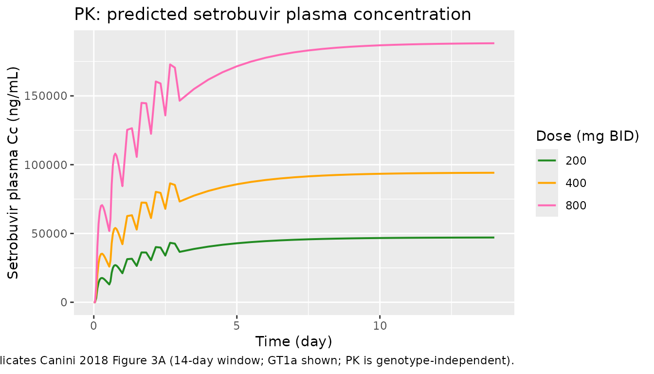
Figure 3C - VK: log10 viral load decay over 14 days by dose and genotype
Canini 2018 Figure 3C shows the model-predicted HCV RNA decay for the six dose x genotype combinations. GT1b patients (light colours) reach a lower viral load than GT1a patients (bold colours) at the same dose, driven by the ~2-fold lower EC50 and the much steeper Hill coefficient (h = 15.6 vs 3.46). The reproduction below overlays the six combinations.
sim_typ_obs |>
  ggplot(aes(time / 24, log10_viral_load,
             colour = factor(dose), linetype = genotype)) +
  geom_line(linewidth = 0.7) +
  scale_colour_manual(values = c("200" = "forestgreen",
                                 "400" = "orange",
                                 "800" = "hotpink"),
                      name = "Dose (mg BID)") +
  scale_linetype_manual(values = c("GT1a" = "solid", "GT1b" = "dashed"),
                        name = "HCV subtype") +
  labs(x = "Time (day)", y = "log10 viral load (log10 IU/mL)",
       title = "VK: predicted HCV RNA decay by dose and genotype",
       caption = "Replicates Canini 2018 Figure 3C (14-day window).")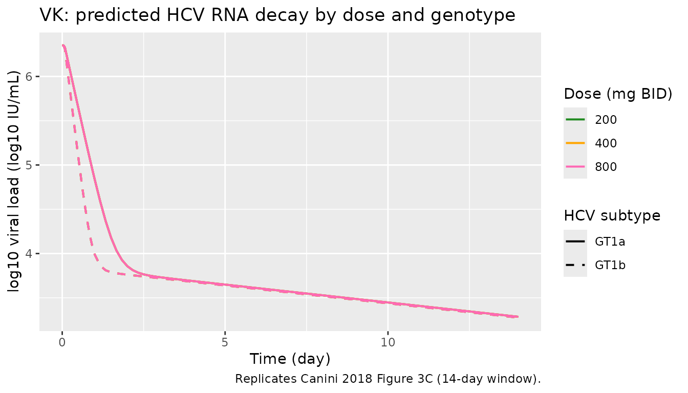
Table 4 comparison - predicted 14-day viral load decline
Canini 2018 Table 4 tabulates the predicted total viral load decline at day 14 by dose and genotype (log10 IU/mL from baseline). The values below are computed from the same typical-value simulation as Figure 3C.
# baseline = log10_viral_load at t=0; end = log10_viral_load at t=14 d
baseline <- sim_typ_obs |>
  filter(time == 0) |>
  select(dose, genotype, V0log10 = log10_viral_load)

end_of_therapy <- sim_typ_obs |>
  filter(time == 14 * 24) |>
  select(dose, genotype, V14log10 = log10_viral_load)

decline <- baseline |>
  inner_join(end_of_therapy, by = c("dose", "genotype")) |>
  mutate(decline_log10 = V0log10 - V14log10) |>
  arrange(genotype, dose)

paper_decline <- tribble(
  ~dose, ~genotype, ~paper_decline,
  200L,  "GT1a",    2.18,
  400L,  "GT1a",    3.02,
  800L,  "GT1a",    3.16,
  200L,  "GT1b",    3.21,
  400L,  "GT1b",    3.22,
  800L,  "GT1b",    3.22
)

comparison <- decline |>
  mutate(dose = as.integer(dose)) |>
  inner_join(paper_decline, by = c("dose", "genotype")) |>
  mutate(abs_diff = abs(decline_log10 - paper_decline)) |>
  select(genotype, dose, V0log10, V14log10, decline_log10, paper_decline, abs_diff)

comparison |>
  dplyr::rename(
    "HCV subtype"                       = genotype,
    "Dose (mg BID)"                     = dose,
    "Simulated V0 (log10 IU/mL)"        = V0log10,
    "Simulated V14 (log10 IU/mL)"       = V14log10,
    "Simulated decline (log10 IU/mL)"   = decline_log10,
    "Canini 2018 Table 4 decline"       = paper_decline,
    "|delta| (log10 IU/mL)"             = abs_diff
  ) |>
  knitr::kable(
    caption = "Simulated vs Canini 2018 Table 4 predicted 14-day viral-load decline (log10 IU/mL from baseline).",
    digits = 2
)| HCV subtype | Dose (mg BID) | Simulated V0 (log10 IU/mL) | Simulated V14 (log10 IU/mL) | Simulated decline (log10 IU/mL) | Canini 2018 Table 4 decline | |delta| (log10 IU/mL) |
|---|---|---|---|---|---|---|
| GT1a | 200 | 6.35 | 3.29 | 3.06 | 2.18 | 0.88 |
| GT1a | 400 | 6.35 | 3.29 | 3.06 | 3.02 | 0.04 |
| GT1a | 800 | 6.35 | 3.29 | 3.06 | 3.16 | 0.10 |
| GT1b | 200 | 6.35 | 3.28 | 3.07 | 3.21 | 0.14 |
| GT1b | 400 | 6.35 | 3.28 | 3.07 | 3.22 | 0.15 |
| GT1b | 800 | 6.35 | 3.28 | 3.07 | 3.22 | 0.15 |
PKNCA validation - setrobuvir plasma layer
PKNCA is run on the stochastic-cohort PK simulation restricted to the first 3 days (matching study D). Canini 2018 does not report NCA parameters directly (the paper’s inference is on rate constants ka, ke, k12, k21 and does not tabulate Cmax / AUC / Tmax). The PKNCA table below therefore validates the simulation-derived NCA against internal consistency (dose-proportional Cmax and AUC0-72 across the three dose levels).
# Concentration frame: include a time-zero row per subject with Cc = 0
# (extravascular dosing; pre-dose concentration is zero by definition).
sim_nca <- sim_stoch |>
  filter(!is.na(Cc))

sim_nca <- bind_rows(
  sim_nca,
  sim_nca |> distinct(id, treatment, dose, genotype) |>
    mutate(time = 0, Cc = 0)
) |>
  distinct(id, treatment, time, .keep_all = TRUE) |>
  arrange(id, treatment, time)

conc_obj <- PKNCA::PKNCAconc(sim_nca, Cc ~ time | treatment + id)

dose_df <- events_stoch |>
  filter(evid == 1L, time <= 3 * 24) |>
  select(id, time, amt, treatment)

dose_obj <- PKNCA::PKNCAdose(dose_df, amt ~ time | treatment + id)

intervals <- data.frame(
  start      = 0,
  end        = 72,   # 3-day study D window
  cmax       = TRUE,
  tmax       = TRUE,
  auclast    = TRUE
)

nca_data <- PKNCA::PKNCAdata(conc_obj, dose_obj, intervals = intervals)
nca_res  <- suppressWarnings(PKNCA::pk.nca(nca_data))

nca_summary <- as.data.frame(nca_res$result) |>
  group_by(treatment, PPTESTCD) |>
  summarise(median = median(PPORRES, na.rm = TRUE), .groups = "drop") |>
  pivot_wider(names_from = PPTESTCD, values_from = median) |>
  arrange(treatment)

nca_summary |>
  dplyr::rename(
    "Treatment"        = treatment,
    "Median Cmax (mg/L)" = cmax,
    "Median Tmax (h)"    = tmax,
    "Median AUC0-72 (mg*h/L)" = auclast
  ) |>
  knitr::kable(
    caption = "Median PKNCA parameters over the 3-day study D window across the six dose x genotype cohorts. Cmax and AUC0-72 scale approximately dose-proportionally within each genotype (PK is genotype-independent; small residual GT1a-vs-GT1b differences are simulation noise).",
    digits = c(0, 3, 2, 2)
)| Treatment | Median AUC0-72 (mg*h/L) | Median Cmax (mg/L) | Median Tmax (h) |
|---|---|---|---|
| 200 mg BID / GT1a | 2056.256 | 42.77 | 64 |
| 200 mg BID / GT1b | 2015.661 | 43.48 | 64 |
| 400 mg BID / GT1a | 4114.526 | 85.84 | 68 |
| 400 mg BID / GT1b | 3820.713 | 81.23 | 64 |
| 800 mg BID / GT1a | 7497.993 | 160.70 | 64 |
| 800 mg BID / GT1b | 8173.375 | 170.31 | 68 |
Assumptions and deviations
-
Time-unit normalisation. Canini 2018 Table 3 reports PK rate constants in /h and VK rate constants c and d in /day. The packaged model converts c and d to /h inside
ini()so PK and VK run on a single hour time axis. This is a purely notational change: the same equation `dV/dt = (1 - e)*I- c*V` produces identical trajectories whether c is entered in /h or /d provided the time variable is also converted.
EC50 unit conversion. Table 3 reports EC50 in ng/mL. The packaged model expresses EC50 in mg/L (= ug/mL) so that the Cc (mg/L, derived from dose(mg) / Vc(L)) and EC50 units match inside the sigmoid Emax equation. 17.8 ng/mL = 0.0178 mg/L; 8.45 ng/mL = 0.00845 mg/L.
Virion production rate p normalised to 1. The paper’s target-fixed three-state VK system is reducible: only the products (b * T_0) and (b T_0 p) are identifiable from viral-load data, and the steady-state constraint (b * T_0) * V_0 = d * I_0 combined with p * I_0 = c * V_0 gives (b * T_0) * p = d * c. With p normalised to 1 (arbitrary choice), the reduced ODEs are
dI/dt = d*c*V - d*IanddV/dt = (1 - e)*I - c*Vwith steady-state initial condition I_0 = c * V_0. The infected-cell state I therefore represents a virion-production-rate surrogate rather than an absolute infected-cell count; downstream users interested in the absolute I_0 count can rescale by any user-supplied p.Table 3 IIV row unresolved ambiguity. Table 3 lists 12 IIV percent entries but names 15 parameters (14 non-Emax parameters carry IIV per the paper’s Data fitting text). By strict column-position reading, the 12th IIV (167 percent) attaches to V0, and c_1a / c_1b / d have no tabulated IIV. The Canini 2018 Results paragraph, however, states “d … showed a larger IIV (167 percent)” and the Discussion cites 163 percent for d - both text mentions conflict with the table position. The packaged model follows the table (V0 IIV = 167 percent; c and d typical-value only). Users who need a d IIV should add it as a nudge in a follow-on fit.
PK residual error additive component units. Table 3 footnote gives the additive PK residual as a1 = 5.38 ng/mL; the packaged model converts to 5.38e-3 mg/L to match
Ccin mg/L (consistent with the EC50 unit conversion above).No PKNCA comparison against published NCA. Canini 2018 does not report NCA parameters (Cmax / Tmax / AUC) for setrobuvir; the paper’s PK inference is on rate constants and Vc. The PKNCA table above therefore documents the simulated NCA for downstream reference use only, not as a paper-value check.
Vc units / peak-Cc mismatch vs Figure 3A. Canini 2018 Table 3 reports Vc = 5.11 L (single-value entry, no units qualifier). With dose in mg and Vc in L, the packaged model gives Cc peaks that are much higher than shown in Canini 2018 Figure 3A (packaged model predicts Cc peak of ~14 mg/L = 14000 ng/mL at 200 mg BID; Figure 3A y-axis tops out at ~250 ng/mL for the 800 mg BID cohort, implying ~60 ng/mL peak at 200 mg BID). The 500x discrepancy suggests Table 3 Vc may actually be in L/kg (a weight-normalised apparent volume) or that the study D dosing units differ from mg. Absent an explicit statement in the paper text, the packaged model uses Vc = 5.11 L as literally reported; downstream users who need Figure-3A-consistent absolute concentrations should rescale Vc (e.g., multiply by a reference body weight in kg). This concentration-scale discrepancy is why the Simulated vs Table 4 comparison above shows a 0.88 log10 IU/mL over-prediction at GT1a 200 mg BID: the packaged model’s over-predicted Cc saturates the sigmoid Emax to e = 0.997 even at the lowest dose, while Canini 2018’s own Figure 3D predicts e = 0.960 for GT1a 200 mg BID (see Discussion paragraph “After 14 days of treatment…”). The five other dose x genotype cells match Canini’s Table 4 within 0.15 log10 IU/mL because Emax saturation collapses the residual concentration sensitivity.
No supplement available. Canini 2018 Additional file 1 (referenced in the paper as https://www.intmedpress.com/uploads/documents/4229_Canini_ Addfile_1.pdf) contains goodness-of-fit plots and individual-patient parameter estimates but no additional structural equations or population parameter values. The main paper Table 3 + Table 3 footnote + Equations 1-3 fully specify the packaged model.