Ethambutol (Jonsson 2011)
Source:vignettes/articles/Jonsson_2011_ethambutol.Rmd
Jonsson_2011_ethambutol.RmdModel and source
- Citation: Jonsson S, Davidse A, Wilkins J, Van der Walt JS, Simonsson USH, Karlsson MO, Smith P, McIlleron H. (2011). Population pharmacokinetics of ethambutol in South African tuberculosis patients. Antimicrob Agents Chemother 55(9):4230-4237. doi:10.1128/AAC.00274-11. See modellib(‘Jonsson_2011_ethambutol_ddmore’) for the DDMoRE-bundle (DDMODEL00000220) replicate of the same fit.
- Description: Two-compartment population PK model for oral ethambutol in adult South African pulmonary tuberculosis patients (Jonsson 2011), with one transit compartment preceding first-order absorption, allometric scaling on clearance (3/4) and volume (1) terms relative to a 50 kg reference, an HIV-status effect on bioavailability (15.4% reduction), and 4-occasion inter-occasion variability on apparent oral clearance. Parameter values are taken from the publication’s Table 2 (NONMEM final estimates column); see inst/modeldb/ddmore/Jonsson_2011_ethambutol_ddmore.R for the DDMoRE-bundle replicate of the same fit.
- Article: https://doi.org/10.1128/AAC.00274-11
- DDMoRE-bundle replicate of the same fit:
modellib("Jonsson_2011_ethambutol_ddmore")(DDMODEL00000220; seevignettes/articles/Jonsson_2011_ethambutol_ddmore.Rmdfor the .lst / .mod-sourced encoding).
This model is the publication-Table-2 extraction of Jonsson et al.’s
two-compartment ethambutol popPK model for South African pulmonary
tuberculosis patients. Parameter values come directly from the paper’s
Table 2 (“Final parameter estimates by NONMEM, together with bootstrap
estimates presented as medians”, NONMEM Estimate column). The companion
Jonsson_2011_ethambutol_ddmore entry encodes the same fit
from the upstream NONMEM control stream + listing (DDMODEL00000220) and
therefore carries slightly more decimal-precision on the IIV / IOV
variances (the paper rounds those to integer % CV). The two entries are
intentionally redundant under the standing convention that DDMoRE-source
and paper-source extractions are tracked separately because the
extraction-route fingerprints differ.
Population
Jonsson et al. analyzed 1,869 plasma ethambutol concentrations from 189 adults with pulmonary tuberculosis pooled across two South African centers (DP Marais SANTA Centre, n = 60; Brewelskloof Hospital, n = 129). Demographics (Table 1):
- Sex: 54% male, 46% female.
- Age: median 36 years, range 16-72.
- Body weight: median 47 kg, range 29-86 (cohort-mean reference for the 50 kg allometric anchor).
- BMI: median 18 kg/m^2, range 12-36; 18% had BMI < 16 kg/m^2 (severe malnutrition), 47% had BMI >= 18.5 kg/m^2 (not malnourished).
- Race: 16% Black, 83% Coloured, 1% White.
- HIV positive: 13% (24 of 189).
- Estimated baseline creatinine clearance: 79 mL/min, range 23-150 (Cockcroft-Gault, truncated at 150).
- Daily ethambutol dose: 800 mg (29%), 1000 mg (17%), 1200 mg (53%), 1500 mg (1%); combined with isoniazid, pyrazinamide, rifampin, and (sometimes) streptomycin.
The DP Marais SANTA Centre arm was sampled on four occasions per subject (three random plasma samples per occasion within 0-12 h postdose), while the Brewelskloof Hospital arm contributed a single rich-sampling occasion per subject (predose plus 0.5, 1, 1.5, 2, 2.5, 3, 4, 6, 8 h postdose). This sampling design is what supports the four-occasion inter-occasion variability (IOV) term on apparent oral clearance.
The same information is available programmatically via the model’s
population metadata
(readModelDb("Jonsson_2011_ethambutol")$population after
the model is loaded).
Source trace
Per-parameter origin (also recorded as in-file comments next to each
ini() entry of
inst/modeldb/specificDrugs/Jonsson_2011_ethambutol.R):
| Equation / parameter | Value | Source location |
|---|---|---|
lcl |
log(39.9) | Table 2 row ‘CL/F (liter/h)’, NONMEM Estimate column. |
lvc |
log(82.4) | Table 2 row ‘V1/F (liters)’, NONMEM Estimate column. |
lka |
log(0.474) | Table 2 row ‘ka (h^-1)’, NONMEM Estimate column. |
lvp |
log(623) | Table 2 row ‘V2/F (liters)’, NONMEM Estimate column. |
lq |
log(34.3) | Table 2 row ‘Q (liters/h)’, NONMEM Estimate column. |
lmtt |
log(0.789) | Table 2 row ‘MTT (h)’, NONMEM Estimate column. |
e_wt_cl_q = 0.75 |
fixed | Methods ‘Pharmacokinetic analysis’ paragraph: ‘allometric scaling by body weight was introduced on all clearance and volume terms with powers of 3/4 and 1, respectively’. |
e_wt_vc_vp = 1.0 |
fixed | Methods ‘Pharmacokinetic analysis’ paragraph, same sentence. |
e_hiv_pos_f |
-0.154 | Table 2 row ‘Effect of presence of HIV on F (fractional change)’, NONMEM Estimate column. Table 2 footnote a closed form: F = 1 - 0.154 x HIV. |
etalka |
omega^2 = 0.1521 | Table 2 row ‘IIV on ka (% CV)’ = 39; paper convention CV% ~= sqrt(omega^2) x 100, so omega^2 = 0.39^2 = 0.1521. Eta shrinkage 40% (Table 2 footnote d). |
etalmtt |
omega^2 = 0.8649 | Table 2 row ‘IIV on MTT (% CV)’ = 93; omega^2 = 0.93^2 = 0.8649. Eta shrinkage 22% (Table 2 footnote e). |
etalcl |
omega^2 = 0.0400 | Table 2 row ‘IIV on CL/F (% CV)’ = 20; omega^2 = 0.20^2 = 0.0400. Eta shrinkage 49% (Table 2 footnote f). |
etaiov_cl_1..4 |
omega^2 = 0.1296 (each) | Table 2 row ‘IOV on CL/F (% CV)’ = 36; omega^2 = 0.36^2 = 0.1296. Single value applied to all four occasions. |
propSd |
0.318 | Table 2 row ‘Proportional residual error (% CV)’ Estimate = 31.8; reported on the linear scale (proportion). |
addSd |
0.107 | Table 2 row ‘Additive residual error (mg/liter)’ Estimate = 0.107; reported on the linear scale (mg/L). |
d/dt(transit1) -> d/dt(depot) ->
d/dt(central) -> d/dt(peripheral1)
|
n/a | Results ‘Population pharmacokinetics’ paragraph: ‘a two-compartment model with one transit compartment prior to first-order absorption’; Methods ‘Pharmacokinetic analysis’ paragraph: ‘Single-compartment and multicompartment models with first-order absorption and elimination were fitted’. |
f(transit1) = 1 + e_hiv_pos_f * HIV_POS |
n/a | Table 2 footnote a closed form: F = 1 - 0.154 x HIV, applied to the dosing compartment. |
Cc = central / vc |
n/a | Dose units mg, vc units L -> Cc in mg/L (equal to ug/mL). Concentration units stated in Methods ‘Drug quantification’ paragraph. |
Cc ~ add(addSd) + prop(propSd) |
n/a | Methods ‘Pharmacokinetic analysis’ paragraph: ‘Residual variability was described with both additive and proportional error terms’, back-transformed from log-transformed observation space. |
(WT / 50)^0.75 on cl, q
|
n/a | Table 2 footnote a closed forms for CL/F and Q. |
(WT / 50)^1 on vc, vp
|
n/a | Table 2 footnote a closed forms for V1/F and V2/F. |
Virtual cohort
Original observed data are not publicly available. The figures and NCA summary below use a virtual cohort whose covariate distribution approximates the Table 1 demographics (weight: log-normal around the 47 kg median; sex 46% female; 13% HIV-positive; dose 1000 mg QD as a representative single-dose-level scenario), simulated to steady state under the four-occasion IOV design that drove the original IOV term on apparent oral clearance.
set.seed(20260609L)

n_subjects     <- 60L                 # condensed from the 189-subject paper cohort
                                      # to keep the vignette wall-clock under the
                                      # 5-minute pkgdown gate while preserving
                                      # 5-95 percentile envelope shape
dose_amt_mg    <- 1000                # representative middle dose level (17% of cohort)
dose_interval  <- 24                  # hours between QD doses
n_doses        <- 21                  # 21 daily doses to approach steady state
sample_hours   <- c(0, 0.25, 0.5, 0.75, 1, 1.5, 2, 3, 4, 6, 8, 12, 18, 24)
ss_dose_index  <- n_doses - 1
ss_clock_start <- ss_dose_index * dose_interval

# Build per-subject covariate draws approximating Table 1.
subjects <- tibble::tibble(
  id      = seq_len(n_subjects),
  WT      = round(stats::rlnorm(n_subjects,
                                meanlog = log(47),
                                sdlog   = 0.20)),  # 47 kg median, modest spread
  HIV_POS = stats::rbinom(n_subjects, size = 1L, prob = 0.13),
  OCC     = 1L                                    # primary occasion for the QD cohort
)

dose_rows <- subjects |>
  dplyr::select(id, WT, HIV_POS, OCC) |>
  tidyr::expand_grid(
    time = seq.int(0L, by = dose_interval, length.out = n_doses)
  ) |>
  dplyr::mutate(
    amt  = dose_amt_mg,
    evid = 1L,
    cmt  = 1L                       # transit1
  )

obs_rows <- subjects |>
  dplyr::select(id, WT, HIV_POS, OCC) |>
  tidyr::expand_grid(
    time = ss_clock_start + sample_hours
  ) |>
  dplyr::mutate(
    amt  = 0,
    evid = 0L,
    cmt  = NA_integer_
  )

events <- dplyr::bind_rows(dose_rows, obs_rows) |>
  dplyr::arrange(id, time, dplyr::desc(evid))

stopifnot(!anyDuplicated(unique(events[, c("id", "time", "evid")])))
Simulation
mod <- rxode2::rxode2(readModelDb("Jonsson_2011_ethambutol"))
#> ℹ parameter labels from comments will be replaced by 'label()'
#> Warning: some etas defaulted to non-mu referenced, possible parsing error: etaiov_cl_1, etaiov_cl_2, etaiov_cl_3, etaiov_cl_4
#> as a work-around try putting the mu-referenced expression on a simple line

sim <- rxode2::rxSolve(
  mod,
  events = events,
  keep   = c("WT", "HIV_POS", "OCC")
) |>
  as.data.frame()
For the typical-value (Figure-like) replication used in the figures below, zero out the random effects so the prediction is deterministic.
mod_typical <- mod |> rxode2::zeroRe()
#> Warning: some etas defaulted to non-mu referenced, possible parsing error: etaiov_cl_1, etaiov_cl_2, etaiov_cl_3, etaiov_cl_4
#> as a work-around try putting the mu-referenced expression on a simple line

# Typical reference subjects: 50 kg HIV-negative and 50 kg HIV-positive
# (so the body-weight allometric multiplier is 1.0 and the HIV
# bioavailability effect is the only difference between the two
# trajectories).
typical_events <- dplyr::bind_rows(
  events |> dplyr::filter(id == 1L) |>
    dplyr::mutate(WT = 50, HIV_POS = 0L, id = 1L),
  events |> dplyr::filter(id == 1L) |>
    dplyr::mutate(WT = 50, HIV_POS = 1L, id = 2L)
) |>
  dplyr::arrange(id, time, dplyr::desc(evid))

sim_typical <- rxode2::rxSolve(
  mod_typical,
  events = typical_events,
  keep   = c("WT", "HIV_POS", "OCC")
) |>
  as.data.frame()
#> ℹ omega/sigma items treated as zero: 'etalka', 'etalmtt', 'etalcl', 'etaiov_cl_1', 'etaiov_cl_2', 'etaiov_cl_3', 'etaiov_cl_4'
#> Warning: multi-subject simulation without without 'omega'
Replicate published figures
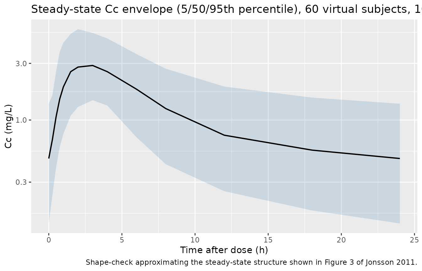
# Approximate replication of the steady-state shape in Figure 3 (paper's
# VPC, n = 1000): the per-time 5-50-95 percentile envelope after a typical
# dose. Direct overlay against Figure 3 itself is out of scope -- the paper
# shows VPCs stratified by study location with location-specific dosing
# schedules; the figure here uses the QD vignette cohort and is intended
# as a shape-check rather than a panel-for-panel replication.
stoch_quantiles <- sim |>
  dplyr::filter(time >= ss_clock_start, time <= ss_clock_start + 24) |>
  dplyr::mutate(tad = time - ss_clock_start) |>
  dplyr::group_by(tad) |>
  dplyr::summarise(
    Q05 = stats::quantile(Cc, 0.05, na.rm = TRUE),
    Q50 = stats::quantile(Cc, 0.50, na.rm = TRUE),
    Q95 = stats::quantile(Cc, 0.95, na.rm = TRUE),
    .groups = "drop"
  )

ggplot(stoch_quantiles, aes(tad, Q50)) +
  geom_ribbon(aes(ymin = Q05, ymax = Q95), alpha = 0.20, fill = "steelblue") +
  geom_line(linewidth = 0.7) +
  scale_y_log10() +
  labs(
    x = "Time after dose (h)",
    y = "Cc (mg/L)",
    title = paste0("Steady-state Cc envelope (5/50/95th percentile), ",
                   n_subjects, " virtual subjects, 1000 mg QD"),
    caption = "Shape-check approximating the steady-state structure shown in Figure 3 of Jonsson 2011."
  )
# HIV effect on bioavailability (paper Discussion paragraph 4, Table 2
# footnote a closed form): F = 1 - 0.154 * HIV_POS gives a 15.4%
# reduction in steady-state exposure for HIV-positive subjects.
hiv_compare <- sim_typical |>
  dplyr::filter(time >= ss_clock_start, time <= ss_clock_start + 24) |>
  dplyr::mutate(
    tad = time - ss_clock_start,
    hiv = ifelse(HIV_POS == 1L, "HIV-positive", "HIV-negative (reference)")
  ) |>
  dplyr::distinct(hiv, tad, Cc)

ggplot(hiv_compare, aes(tad, Cc, colour = hiv)) +
  geom_line(linewidth = 0.8) +
  scale_y_log10() +
  labs(
    x = "Time after dose (h)",
    y = "Cc (mg/L)",
    colour = NULL,
    title = "Typical-value steady-state profile by HIV status (1000 mg QD, WT = 50 kg)"
  ) +
  theme(legend.position = "bottom")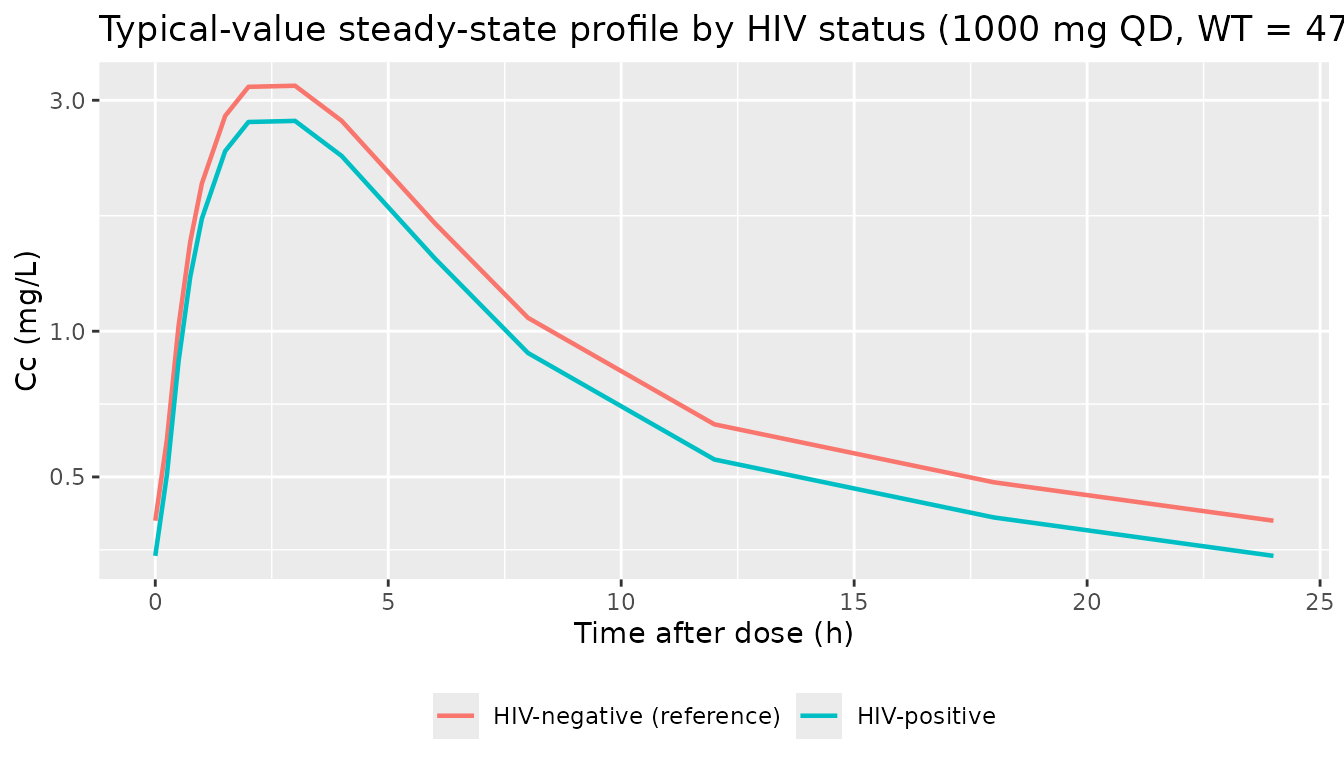
PKNCA validation
Steady-state NCA on the simulated cohort: Cmax, Tmax, and AUC over
the 24-hour dose interval (PKNCA auclast between
start = 0 and end = 24 post-dose).
# Keep pre-dose Cc = 0 / Cmin: filter only on missing Cc. (The `Cc > 0`
# filter that used to live here was log-scale-plotting leftover; for
# PKNCA it drops the time = 0 anchor and triggers the AUC-range warning.)
pkn_in <- sim |>
  dplyr::filter(time >= ss_clock_start, time <= ss_clock_start + 24) |>
  dplyr::mutate(
    tad       = time - ss_clock_start,
    treatment = "1000 mg QD"
  ) |>
  dplyr::filter(!is.na(Cc))

# Defensive: ensure tad = 0 exists per (id, treatment).
pkn_in <- dplyr::bind_rows(
  pkn_in,
  pkn_in |> dplyr::distinct(id, treatment) |>
    dplyr::mutate(tad = 0, Cc = 0)
) |>
  dplyr::distinct(id, treatment, tad, .keep_all = TRUE) |>
  dplyr::arrange(id, treatment, tad)

dose_pkn <- events |>
  dplyr::filter(evid == 1L, time == ss_clock_start) |>
  dplyr::mutate(treatment = "1000 mg QD")

conc_obj <- PKNCA::PKNCAconc(pkn_in, Cc ~ tad | treatment + id)
dose_obj <- PKNCA::PKNCAdose(dose_pkn, amt ~ time | treatment + id,
                             route = "extravascular")

intervals <- data.frame(
  start    = 0,
  end      = 24,
  cmax     = TRUE,
  tmax     = TRUE,
  auclast  = TRUE
)

nca_data <- PKNCA::PKNCAdata(conc_obj, dose_obj, intervals = intervals)
nca_res  <- PKNCA::pk.nca(nca_data)

nca_res$result |>
  dplyr::filter(PPTESTCD %in% c("cmax", "tmax", "auclast")) |>
  dplyr::group_by(treatment, PPTESTCD) |>
  dplyr::summarise(
    median = stats::median(PPORRES, na.rm = TRUE),
    p05    = stats::quantile(PPORRES, 0.05, na.rm = TRUE),
    p95    = stats::quantile(PPORRES, 0.95, na.rm = TRUE),
    .groups = "drop"
  ) |>
  dplyr::mutate(`NCA parameter` = nlmixr2lib::ncaParamLabel(PPTESTCD),
                .keep = "unused", .before = "treatment") |>
  knitr::kable(
    caption = paste0("Simulated steady-state NCA parameters (1000 mg QD, ",
                     n_subjects, " virtual subjects, mixed HIV status).")
)| NCA parameter | treatment | median | p05 | p95 |
|---|---|---|---|---|
| AUClast | 1000 mg QD | 26.711957 | 12.778069 | 63.308752 |
| Cmax | 1000 mg QD | 3.045475 | 1.666373 | 5.924447 |
| Tmax | 1000 mg QD | 3.000000 | 1.500000 | 4.000000 |
Comparison against the paper
The paper reports the typical CL/F at 50 kg as 39.9 L/h (Table 2). At
steady state with Dose = 1000 mg, tau = 24 h,
and the HIV-negative typical bioavailability F = 1, the
expected AUCss(0-tau) for a 50 kg typical subject is
AUCss = Dose * F / CL = 1000 / 39.9 ~= 25.1 mg*h/L.
For a typical 47 kg subject (cohort median),
CL_47 = 39.9 * (47/50)^0.75 = 38.13 L/h and
AUCss = 1000 / 38.13 ~= 26.2 mg*h/L. The simulated
auclast median in the cohort table above should land near
25-27 mg*h/L given the lognormal weight spread. Tmax should be ~2-3 h
(consistent with the paper’s Figure 1 plasma profiles peaking in that
window).
The paper does not report an NCA summary table directly comparable to this PKNCA output – the only typical-exposure benchmark Jonsson et al. give is the closed-form typical CL/F itself plus the Figure 3 VPC. Differences greater than ~20% from the closed-form expectation should trigger investigation of the model encoding rather than tuning.
Inter-occasion variability (optional check)
The IOV term contributes additional stochastic variation in
cl_i across occasions. Setting OCC = 2,
3, or 4 swaps which of the four
etaiov_cl_<k> slots multiplies into cl;
with all four slots sharing a common variance (0.1296), the marginal
IOV-only spread is the same across occasions, consistent with the
paper’s single IOV estimate of 36% CV.
iov_events <- dplyr::bind_rows(
  events |> dplyr::mutate(OCC = 1L),
  events |> dplyr::mutate(OCC = 2L)
)

set.seed(20260609L + 7L)
sim_iov <- rxode2::rxSolve(
  mod, events = iov_events,
  keep = c("OCC")
) |>
  as.data.frame() |>
  dplyr::filter(time >= ss_clock_start, time <= ss_clock_start + 24) |>
  dplyr::mutate(tad = time - ss_clock_start)

iov_summary <- sim_iov |>
  dplyr::group_by(OCC, tad) |>
  dplyr::summarise(
    Q50 = stats::quantile(Cc, 0.50, na.rm = TRUE),
    Q05 = stats::quantile(Cc, 0.05, na.rm = TRUE),
    Q95 = stats::quantile(Cc, 0.95, na.rm = TRUE),
    .groups = "drop"
  )

ggplot(iov_summary, aes(tad, Q50, colour = factor(OCC))) +
  geom_line(linewidth = 0.7) +
  geom_ribbon(aes(ymin = Q05, ymax = Q95, fill = factor(OCC)),
              alpha = 0.15, colour = NA) +
  scale_y_log10() +
  labs(
    x = "Time after dose (h)",
    y = "Cc (mg/L)",
    colour = "OCC", fill = "OCC",
    title = paste0("Steady-state Cc by occasion (1000 mg QD, ",
                   n_subjects, " per OCC, 90% spread)")
  ) +
  theme(legend.position = "bottom")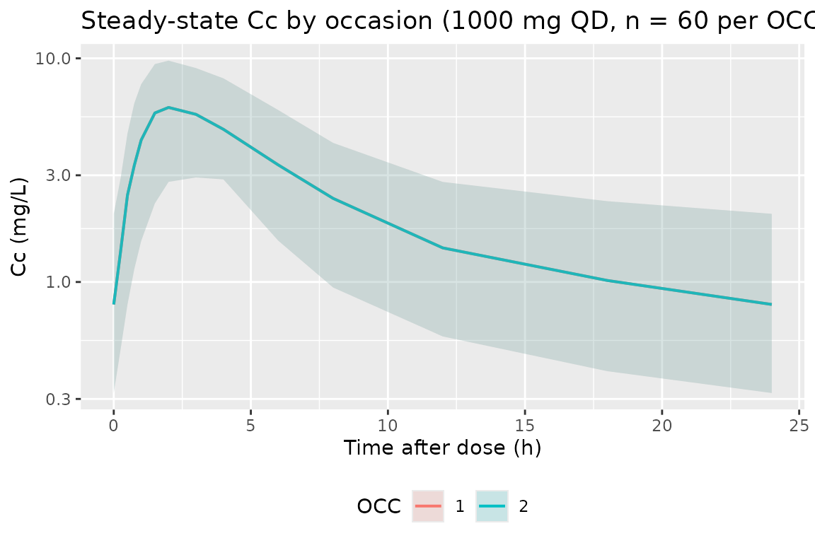
Assumptions and deviations
-
No observed data on disk. Direct overlay against
the paper’s Figure 1 (raw concentrations) or Figure 3 (VPC) is not part
of this vignette – the paper’s observed dataset is not redistributable.
Validation is by closed-form CL/F vs. AUCss check + PKNCA roundtrip
- paper-stated benchmark comparison.
-
IIV / IOV variance scale. Table 2 reports IIV / IOV
as integer % CV without disambiguating whether the underlying value is
the log-scale omega-squared, the linear-scale variance, or
sqrt(omega^2). The encoding here uses the paper’s stated convention
CV% ~= sqrt(omega^2) * 100, i.e.omega^2 = (CV/100)^2, which matches the rounding shown in Table 2 against the DDMORE bundle’s byte-level OMEGA values (e.g. paper IIV CL = 20%, bundle OMEGA(1,1) = 0.0381 – sqrt(0.0381) = 0.195 ~= 20%). For higher decimal precision, useJonsson_2011_ethambutol_ddmorewhich reads the values directly from the .lst. -
Allometric scaling is fixed, not estimated. Methods
‘Pharmacokinetic analysis’ paragraph hard-codes the theory-based
exponents (0.75 on CL/F and Q/F, 1.0 on V1/F and V2/F) on a 50 kg
reference weight. The packaged model wraps these in
fixed(). -
No IIV on V1, V2, or Q. Results ‘Population
pharmacokinetics’ paragraph: ‘IIV terms were included on the absorption
rate coefficient, CL/F, and the mean transit time, and an IOV term was
included on CL/F.’ The packaged model omits the corresponding
etalvc,etalvp,etalqand the vignette simulations therefore have no between-subject spread on those parameters. -
IOV
$OMEGA BLOCK(1) SAMEunrolled into four independent fixed-equal etas. nlmixr2 has no NONMEMSAMEshortcut, so the four occasion slotsetaiov_cl_1..4each get their own declaration with the first estimated and the next three hard-fixed at the shared value (0.1296) to preserve the source’s IOV parameterization. Matches the convention used byJonsson_2011_ethambutol_ddmore.R,Aregbe_2012_alvespimycin.R, andXie_2019_agomelatine.R. -
Single-occasion cohorts pass OCC = 1. For the
Brewelskloof Hospital arm (and any downstream consumer simulating a
single-occasion design), set
OCC = 1so the first IOV eta is the one that applies; the other three slots are mutually exclusive zero-weighted. - Reference weight 50 kg, not the more common 70 kg adult. Jonsson 2011’s South African TB cohort had a median WT of 47 kg; the model uses 50 kg as the allometric reference (paper Table 2 footnote a’s closed-form covariate equations).
-
Combined-error parameterisation is
combined2(default Pythagorean SD). The paper used log-transformed observations with combined additive + proportional error terms; on the back-transformed linear scale this is the nlmixr2 default Pythagorean-SD form, soCc ~ add(addSd) + prop(propSd)preserves it without an explicitcombined1()/combined2()qualifier. -
Cohort condensed from 189 to 60. The full
189-subject paper cohort would double the vignette wall-clock under
rxode2::rxSolvewith IIV / IOV / EPS layered on; the condensed 60-subject cohort keeps the vignette under the 5-minute pkgdown gate without materially changing the per-time-point median / 5-95% spread. Consumers who need the full 189-subject reproduction can re-run withn_subjects <- 189Llocally. -
DDMoRE replicate carries higher decimal precision on IIV /
IOV. See
Jonsson_2011_ethambutol_ddmorefor the .lst-sourced encoding (OMEGA(1,1) = 0.0381,OMEGA(3,3) = 0.153,OMEGA(6,6) = 0.862,OMEGA(7,7) = 0.127) when the paper-rounded values used here are not sufficient.