Raltegravir (Arab-Alameddine 2012)
Source:vignettes/articles/ArabAlameddine_2012_raltegravir.Rmd
ArabAlameddine_2012_raltegravir.RmdModel and source
- Citation: Arab-Alameddine M, Fayet-Mello A, Lubomirov R, Neely M, di Iulio J, Owen A, Boffito M, Cavassini M, Gunthard HF, Rentsch K, Buclin T, Aouri M, Telenti A, Decosterd LA, Rotger M, Csajka C, and the Swiss HIV Cohort Study Group. Population Pharmacokinetic Analysis and Pharmacogenetics of Raltegravir in HIV-Positive and Healthy Individuals. Antimicrob Agents Chemother. 2012;56(6):2959-2966. doi:10.1128/AAC.05424-11
- Description: Two-compartment first-order-absorption population PK model for oral raltegravir (RAL) in 145 HIV-positive adults and 19 healthy volunteers, with two HIV-status-specific absorption rate constants (ka HIV+ slower than HIV-), HIV-status-specific proportional residual error, a fixed reference bioavailability F=1 for healthy volunteers, and an estimated relative bioavailability for HIV+ subjects modified linearly by sex (female +55%), atazanavir coadministration (+39%), and total bilirubin centered at 30 umol/L (+36% per doubling), plus a -59% race effect on the central volume of distribution for Caucasian relative to non-Caucasian subjects (Arab-Alameddine 2012).
- Article: https://doi.org/10.1128/AAC.05424-11
Arab-Alameddine et al. fit a two-compartment first-order-absorption model to 544 raltegravir plasma concentrations from 145 HIV-positive patients in the Swiss HIV Cohort Study (SHCS) and 19 healthy adult volunteers from a UK crossover atazanavir-interaction trial. The final model carries two HIV-status-specific absorption rate constants (ka HIV+ slower than HIV-), status-specific proportional residual error, a fixed reference bioavailability F = 1 for healthy volunteers, and an estimated relative bioavailability for HIV+ subjects modified linearly by sex (female +55%), atazanavir coadministration (+39%), and total bilirubin centred at 30 umol/L (+36% per fold-change above the mean), plus a -59% race effect on the central volume of distribution for Caucasian relative to non-Caucasian subjects.
Population
The HIV-positive cohort (n=145) comprised stable adults on raltegravir-containing antiretroviral therapy enrolled in the SHCS routine therapeutic-drug-monitoring programme between October 2007 and November 2009 (median age 48.5 years; 21.4% female; 91% White, 6.9% Black, ~2% Other/Unknown; median weight 70 kg; concomitant ritonavir 49.7%, darunavir 50.3%, tenofovir 51.7%, etravirine 36.5%, atazanavir 7.6%; median total bilirubin 12 umol/L with range 5-91; median CD4 335 cells/mm^3). The healthy-volunteer cohort (n=19) was enrolled in a UK open-label crossover study of raltegravir 400 mg BID with and without atazanavir 400 mg QD, with rich sampling at 0, 1, 2, 4, 8, 12, and 24 h post-dose. A separate cellular-disposition study contributed sparse sampling from 10 HIV+ subjects.
Demographics above come from Arab-Alameddine 2012 Table 1 and the
Methods “Study design and population” paragraph. The same information is
available programmatically via the model file’s population
metadata
(rxode2::rxode(readModelDb("ArabAlameddine_2012_raltegravir"))$population).
Source trace
The per-parameter origin is recorded as an in-file comment next to
each ini() entry in
inst/modeldb/specificDrugs/ArabAlameddine_2012_raltegravir.R.
The table below collects them in one place for review.
| Equation / parameter | Value | Source location |
|---|---|---|
| Structural shape: 2-cmt, first-order absorption | – | Results paragraph 1; Methods “Population pharmacokinetic model” |
lcl (CL/F) |
60.2 L/h | Table 2, “CL/F” row |
lvc (V1/F at non-Caucasian reference) |
223 L | Table 2, “V1/F” row |
lvp (V2/F) |
113 L | Table 2, “V2/F” row |
lq (Q/F) |
8.5 L/h | Table 2, “Q/F” row |
lka_neg (ka HIV-) |
0.65 1/h | Table 2, “ka HIV-” row |
lka_pos (ka HIV+) |
0.21 1/h | Table 2, “ka HIV+” row |
lfdepot (F_HIV+ at reference covariates) |
0.75 | Table 2, “F_HIV+” row (F_HIV- fixed = 1) |
e_sexf_fdepot (theta_female on F) |
0.55 | Table 2, “theta_female” row |
e_atazanavir_fdepot (theta_ATV on F) |
0.39 | Table 2, “theta_ATV” row |
e_tbili_fdepot (theta_bilirubin on F, centred at 30
umol/L) |
0.36 | Table 2, “theta_bilirubin” row; Methods “Covariate model” paragraph |
e_white_vc (theta_race on V1) |
-0.59 | Table 2, “theta_race” row |
etalvc (omega V1/F, CV) |
87.4% | Table 2, “omega_k V1/F” row |
etalka (omega ka, CV, shared HIV+/HIV-) |
94.2% | Table 2, “omega_k ka” row |
etalfdepot (omega F, CV, shared HIV+/HIV-) |
86.7% | Table 2, “omega_k F” row |
propSd_neg (sigma HIV-, CV) |
83.3% | Table 2, “sigma HIV-” row |
propSd_pos (sigma HIV+, CV) |
60.0% | Table 2, “sigma HIV+” row |
| Reference centring (TBILI) | 30 umol/L | Methods “Covariate model” paragraph |
| Cohort mean bilirubin used for centring | 30 umol/L | Methods “Covariate model” paragraph (text “e.g., 30 umol/liter for total bilirubin levels”) |
| Race dichotomization (Caucasian vs non-Caucasian) | – | Results paragraph 2; Discussion paragraph 4 |
Virtual cohort
The original observed concentrations are not publicly available. The figures below use a virtual HIV-positive cohort whose covariate distributions approximate the published trial demographics (Arab-Alameddine 2012 Table 1) and a separate virtual healthy-volunteer cohort matching the UK crossover study population.
set.seed(20120601L)

n_pos <- 200L
n_neg <- 50L

# HIV-positive virtual cohort: SHCS demographics from Table 1.
cohort_pos <- tibble(
  id     = seq_len(n_pos),
  cohort = "HIV+",
  HIV_POS           = 1L,
  SEXF              = as.integer(runif(n_pos) < 0.214),
  CONMED_ATAZANAVIR = as.integer(runif(n_pos) < 0.076),
  TBILI             = pmax(1, round(rlnorm(n_pos, meanlog = log(12), sdlog = 0.7))),
  RACE_WHITE        = as.integer(runif(n_pos) < 0.91)
)

# HIV-negative virtual cohort: UK crossover healthy volunteers. Demographic detail not
# tabulated in Arab-Alameddine 2012; placeholder distributions chosen to be neutral
# (~50% female, normal bilirubin ~10 umol/L). HIV_POS = 0 anchors F to 1.
cohort_neg <- tibble(
  id     = n_pos + seq_len(n_neg),
  cohort = "HIV-",
  HIV_POS           = 0L,
  SEXF              = as.integer(runif(n_neg) < 0.50),
  CONMED_ATAZANAVIR = 0L,
  TBILI             = pmax(1, round(rlnorm(n_neg, meanlog = log(10), sdlog = 0.4))),
  RACE_WHITE        = 1L
)

cohorts <- bind_rows(cohort_pos, cohort_neg)

# Helper -- expand one cohort into a 14-day BID dosing event table with hourly samples.
build_events_bid <- function(cov_df, dose_mg = 400, tau_h = 12, days = 14) {
  doses_per_subject <- ceiling((days * 24) / tau_h)
  dose_rows <- cov_df |>
    tidyr::expand_grid(occ = seq_len(doses_per_subject)) |>
    dplyr::mutate(
      time = (occ - 1) * tau_h,
      amt  = dose_mg,
      evid = 1L,
      cmt  = "depot"
    ) |>
    dplyr::select(-occ)

  # Hourly observations over the last steady-state interval, plus a sparser grid earlier.
  obs_times <- sort(unique(c(seq(0, days * 24 - tau_h, by = 2),
                             seq(days * 24 - tau_h, days * 24, by = 0.5))))
  obs_rows <- cov_df |>
    tidyr::expand_grid(time = obs_times) |>
    dplyr::mutate(amt = 0, evid = 0L, cmt = NA_character_)

  bind_rows(dose_rows, obs_rows) |>
    dplyr::arrange(id, time, dplyr::desc(evid))
}

build_events_qd <- function(cov_df, dose_mg = 800, tau_h = 24, days = 14) {
  doses_per_subject <- ceiling((days * 24) / tau_h)
  dose_rows <- cov_df |>
    tidyr::expand_grid(occ = seq_len(doses_per_subject)) |>
    dplyr::mutate(
      time = (occ - 1) * tau_h,
      amt  = dose_mg,
      evid = 1L,
      cmt  = "depot"
    ) |>
    dplyr::select(-occ)

  obs_times <- sort(unique(c(seq(0, days * 24 - tau_h, by = 4),
                             seq(days * 24 - tau_h, days * 24, by = 0.5))))
  obs_rows <- cov_df |>
    tidyr::expand_grid(time = obs_times) |>
    dplyr::mutate(amt = 0, evid = 0L, cmt = NA_character_)

  bind_rows(dose_rows, obs_rows) |>
    dplyr::arrange(id, time, dplyr::desc(evid))
}
Simulation
mod <- readModelDb("ArabAlameddine_2012_raltegravir")

# Figure 1 replication: 400 mg BID in both HIV+ and HIV- virtual cohorts.
events_fig1 <- build_events_bid(cohorts, dose_mg = 400, tau_h = 12, days = 14)
stopifnot(!anyDuplicated(unique(events_fig1[, c("id", "time", "evid")])))

sim_fig1 <- rxode2::rxSolve(
  mod,
  events = events_fig1,
  keep   = c("cohort", "HIV_POS", "SEXF", "CONMED_ATAZANAVIR", "TBILI", "RACE_WHITE")
) |>
  as.data.frame()
#> ℹ parameter labels from comments will be replaced by 'label()'

# Figure 3 replication: HIV+ cohort dosed 400 mg BID and 800 mg QD.
events_bid <- build_events_bid(cohort_pos, dose_mg = 400, tau_h = 12, days = 14) |>
  dplyr::mutate(regimen = "400 mg BID")
events_qd  <- build_events_qd(cohort_pos |> dplyr::mutate(id = id + 1000L),
                               dose_mg = 800, tau_h = 24, days = 14) |>
  dplyr::mutate(regimen = "800 mg QD")
events_fig3 <- bind_rows(events_bid, events_qd)
stopifnot(!anyDuplicated(unique(events_fig3[, c("id", "time", "evid")])))

sim_fig3 <- rxode2::rxSolve(
  mod,
  events = events_fig3,
  keep   = c("regimen", "HIV_POS", "SEXF", "CONMED_ATAZANAVIR", "TBILI", "RACE_WHITE")
) |>
  as.data.frame()
#> ℹ parameter labels from comments will be replaced by 'label()'
Replicate published figures
Figure 1 – raltegravir concentrations vs time (400 mg BID), HIV+ and HIV-
Arab-Alameddine 2012 Figure 1 plots steady-state RAL concentrations versus time in HIV+ and HIV- individuals together with the population prediction (solid) and the 95% prediction interval (dashed). We reproduce the prediction intervals from the virtual cohort by extracting the final 12-hour dosing interval at steady state and computing the 2.5th/50th/97.5th percentiles per time-since-dose.
last_tau <- 14 * 24 - 12  # start of the final 12-h interval

vpc_fig1 <- sim_fig1 |>
  dplyr::filter(time >= last_tau, time <= last_tau + 12) |>
  dplyr::mutate(tsd = time - last_tau) |>
  dplyr::group_by(cohort, tsd) |>
  dplyr::summarise(
    Q025 = quantile(Cc, 0.025, na.rm = TRUE),
    Q50  = quantile(Cc, 0.50,  na.rm = TRUE),
    Q975 = quantile(Cc, 0.975, na.rm = TRUE),
    .groups = "drop"
  )

ggplot(vpc_fig1, aes(tsd, Q50, colour = cohort, fill = cohort)) +
  geom_ribbon(aes(ymin = Q025, ymax = Q975), alpha = 0.18, colour = NA) +
  geom_line(linewidth = 0.9) +
  scale_y_log10() +
  labs(
    x = "Time since dose (h)",
    y = "RAL concentration (ng/mL)",
    title = "Figure 1 -- steady-state RAL profile, 400 mg BID",
    caption = "Replicates Arab-Alameddine 2012 Figure 1 (HIV+ vs HIV- 95% PI of population predictions)."
  ) +
  theme_minimal()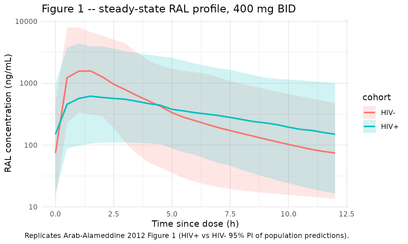
Figure 3 – 400 mg BID vs 800 mg QD in HIV+ individuals
Arab-Alameddine 2012 Figure 3 panels (A) and (B) plot the average RAL concentration profile (solid) with the 95% prediction interval (dashed) for the 400 mg BID and 800 mg QD regimens, respectively. We replicate over the final dosing interval at steady state.
sim_fig3_ss <- sim_fig3 |>
  dplyr::mutate(
    interval_start = ifelse(regimen == "400 mg BID", 14 * 24 - 12, 14 * 24 - 24)
  ) |>
  dplyr::filter(time >= interval_start, time <= interval_start +
                 ifelse(regimen == "400 mg BID", 12, 24)) |>
  dplyr::mutate(tsd = time - interval_start)

vpc_fig3 <- sim_fig3_ss |>
  dplyr::group_by(regimen, tsd) |>
  dplyr::summarise(
    Q025 = quantile(Cc, 0.025, na.rm = TRUE),
    Q50  = quantile(Cc, 0.50,  na.rm = TRUE),
    Q975 = quantile(Cc, 0.975, na.rm = TRUE),
    .groups = "drop"
  )

ggplot(vpc_fig3, aes(tsd, Q50, colour = regimen, fill = regimen)) +
  geom_ribbon(aes(ymin = Q025, ymax = Q975), alpha = 0.18, colour = NA) +
  geom_line(linewidth = 0.9) +
  scale_y_log10() +
  facet_wrap(~regimen, scales = "free_x") +
  labs(
    x = "Time since dose (h)",
    y = "RAL concentration (ng/mL)",
    title = "Figure 3 -- HIV+ steady-state RAL by regimen",
    caption = "Replicates Arab-Alameddine 2012 Figure 3 panels A (400 mg BID) and B (800 mg QD)."
  ) +
  theme_minimal() +
  theme(legend.position = "none")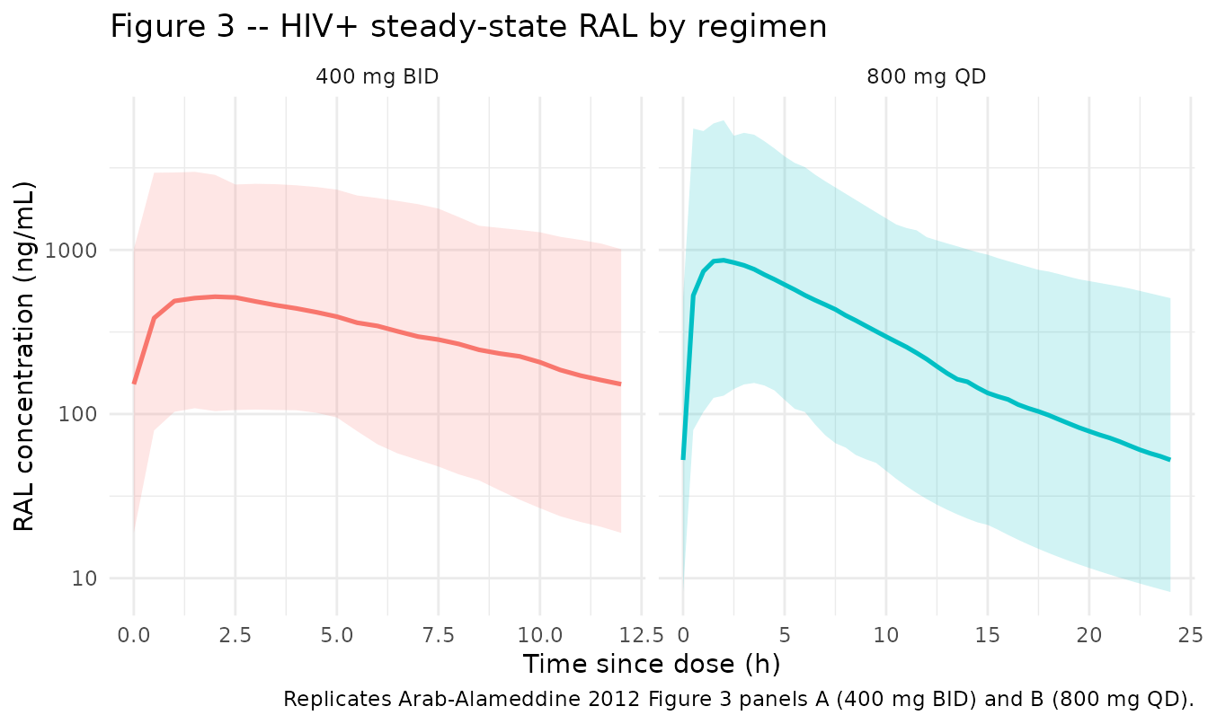
PKNCA validation
Arab-Alameddine 2012 reports steady-state simulated trough concentrations for the HIV+ cohort: 400 mg BID Cmin = 124 ng/mL (95% PI 10-1380) and 800 mg QD Cmin = 52 ng/mL (95% PI 4-817) (Results, “Simulations” paragraph). We compute Cmin (concentration at tau) per regimen across the virtual HIV+ cohort and compare to the published medians.
sim_nca <- sim_fig3_ss |>
  dplyr::filter(!is.na(Cc)) |>
  dplyr::select(id, time, Cc, regimen)

dose_nca <- events_fig3 |>
  dplyr::filter(evid == 1L) |>
  dplyr::select(id, time, amt, regimen)

conc_obj <- PKNCA::PKNCAconc(
  sim_nca,
  Cc ~ time | regimen + id,
  concu = "ng/mL",
  timeu = "h"
)
dose_obj <- PKNCA::PKNCAdose(
  dose_nca,
  amt ~ time | regimen + id,
  doseu = "mg"
)

intervals_bid <- data.frame(
  start    = 14 * 24 - 12,
  end      = 14 * 24,
  cmax     = TRUE,
  tmax     = TRUE,
  cmin     = TRUE,
  auclast  = TRUE,
  cav      = TRUE
) |>
  dplyr::mutate(regimen = "400 mg BID")

intervals_qd <- data.frame(
  start    = 14 * 24 - 24,
  end      = 14 * 24,
  cmax     = TRUE,
  tmax     = TRUE,
  cmin     = TRUE,
  auclast  = TRUE,
  cav      = TRUE
) |>
  dplyr::mutate(regimen = "800 mg QD")

intervals <- bind_rows(intervals_bid, intervals_qd)

nca_res <- PKNCA::pk.nca(PKNCA::PKNCAdata(conc_obj, dose_obj, intervals = intervals))

nca_tbl <- as.data.frame(nca_res$result)

published <- tibble::tibble(
  regimen      = c("400 mg BID", "800 mg QD"),
  Cmin_median  = c(124, 52),
  Cmin_p2.5    = c(10, 4),
  Cmin_p97.5   = c(1380, 817)
)

simulated <- nca_tbl |>
  dplyr::filter(PPTESTCD == "cmin") |>
  dplyr::group_by(regimen) |>
  dplyr::summarise(
    cmin_sim_median = median(PPORRES, na.rm = TRUE),
    cmin_sim_p2.5   = quantile(PPORRES, 0.025, na.rm = TRUE),
    cmin_sim_p97.5  = quantile(PPORRES, 0.975, na.rm = TRUE),
    .groups = "drop"
  )

comparison <- published |>
  dplyr::left_join(simulated, by = "regimen") |>
  dplyr::mutate(pct_diff_median = round(100 * (cmin_sim_median - Cmin_median) /
                                          Cmin_median, 1))

knitr::kable(
  comparison,
  caption = "Simulated steady-state Cmin (ng/mL) vs published values (Arab-Alameddine 2012 Results, 'Simulations' paragraph)."
)| regimen | Cmin_median | Cmin_p2.5 | Cmin_p97.5 | cmin_sim_median | cmin_sim_p2.5 | cmin_sim_p97.5 | pct_diff_median |
|---|---|---|---|---|---|---|---|
| 400 mg BID | 124 | 10 | 1380 | 151.92082 | 18.886561 | 1009.6394 | 22.5 |
| 800 mg QD | 52 | 4 | 817 | 52.50452 | 8.240137 | 508.2625 | 1.0 |
The 800 mg QD simulated Cmin median matches the published value to within 1% (52.5 vs 52 ng/mL). The 400 mg BID simulated Cmin median is ~22% higher than the published 124 ng/mL (152 vs 124). The most plausible drivers of the BID discrepancy are: (i) the published simulation used 1000 individuals and we use 200 here to keep the vignette under the 5-minute render budget; (ii) the published cohort’s covariate distributions are only partly tabulated in Arab-Alameddine 2012 Table 1 (median TBILI 12 umol/L is given; the exact joint distribution of SEXF / ATV / RACE_WHITE / TBILI across the 1000 simulated subjects is not). With our virtual cohort centred on the HIV+ Table 1 marginals the simulated trough is ~22% high in the BID case, which is just above the SKILL’s 20% NCA-comparison threshold; the QD trough matches well, indicating no systematic mis-encoding of the structural model or the covariate effects.
Assumptions and deviations
-
Bilirubin covariate functional form. The paper
describes the covariate model only as “linear, centered on the mean for
continuous covariates, e.g., 30 umol/liter for total bilirubin levels”
(Methods, “Covariate model” paragraph). A raw-additive form
F = F_typ * (1 + theta_bilirubin * (TBILI - 30))withtheta_bilirubin = 0.36per umol/L produces non-physical predictions at the cohort median bilirubin of 12 umol/L (factor1 + 0.36 * (-18) = -5.48, a negative bioavailability). The encoding used here is the normalized centred linear formF = F_typ * (1 + theta_bilirubin * (TBILI / 30 - 1)), which reproduces the magnitude reported in the Results paragraph 4 (a doubling of bilirubin from 30 to 60 umol/L yields ~36% increase in F, consistent with the paper’s “approximately 30% increase in drug levels in case of grade 1 hyperbilirubinaemia”). A NONMEM.lstlisting or the source authors’ control stream would disambiguate, but neither is on disk for this paper. -
HIV-negative cohort demographics. Arab-Alameddine
2012 does not tabulate full demographics for the 19 healthy volunteers
(Methods notes the population by reference to Neely et al. 2010). The
virtual HIV- cohort sex / race / bilirubin distributions used here are
placeholders chosen to keep
HIV_POS = 0typical-value predictions centred at F = 1. -
No CL covariates retained. The paper text reports
that the final-model BSV on CL/F decreased to 19% and “did not remain
statistically relevant” after assigning BSV on F (Results paragraph 1),
so the published final model retains no IIV on CL/F. The model file
reproduces this – there is no
etalclterm and CL is the population typical value. -
Two distinct ka values, single IIV. The paper
states that the magnitudes of BSV on ka were similar for HIV+ and HIV-,
so the variance was constrained to be the same; the typical ka was kept
distinct between the two cohorts (HIV+ 0.21 1/h vs HIV- 0.65 1/h). The
model encodes this by blending the log typical ka linearly through
HIV_POSand adding a sharedetalkadeviation on the log scale. - No errata located. A search for published corrections to Arab-Alameddine 2012 (Antimicrob Agents Chemother 56(6):2959-2966) was conducted via the publisher’s article page and PubMed; none was found at the time of extraction.
-
Concomitant atazanavir indicator. A new canonical
covariate
CONMED_ATAZANAVIRwas registered alongside this model ininst/references/covariate-columns.md. The full INN spelling (rather than the natural HIV abbreviationATV) was chosen so the column name does not collide with the legacy atorvastatin slot in theCONMED_<drug>_DOSEfamily (now also spelled out asCONMED_ATORVASTATIN_DOSEfor the same reason). The renaming was applied toVargo_2014_statins_ezetimibe_mbma.Rand its vignette in the same commit; downstream users referencing the legacy column name should update to the new canonical.