Meropenem (Cojutti 2021)
Source:vignettes/articles/Cojutti_2021_meropenem.Rmd
Cojutti_2021_meropenem.RmdModel and source
- Citation: Cojutti PG, Gatti M, Rinaldi M, Tonetti T, Laici C, Mega C, Siniscalchi A, Giannella M, Viale P, Pea F. Impact of Maximizing Css/MIC Ratio on Efficacy of Continuous Infusion Meropenem Against Documented Gram-Negative Infections in Critically Ill Patients and Population Pharmacokinetic/Pharmacodynamic Analysis to Support Treatment Optimization. Front Pharmacol. 2021;12:781892. doi:10.3389/fphar.2021.781892. PMCID: PMC8694396. Structural and variability estimates are Table 4 (‘Final model’ columns); the covariate equations are printed in Section 3.3; the residual-error polynomial and gamma are in Section 2.4. No supplement was published and no erratum was found (Europe PMC search, 2026-09-30).
- Description: One-compartment population PK model for meropenem given by continuous intravenous infusion to 74 critically ill adults (one adolescent) with Gram-negative infections at a tertiary hospital in Bologna, Italy, fitted non-parametrically with the NPAG algorithm in Pmetrics 1.5.0 to 183 steady-state therapeutic-drug-monitoring concentrations. Clearance is ADDITIVE in an intercept and an arm linear in CKD-EPI creatinine clearance (CL = theta1 + theta2 * CLCR), and volume is a power function of absolute total body weight (V = theta3 * BW^theta4). All four thetas carry inter-individual variability taken from the CVs of the NPAG marginal distributions, including the body-weight exponent. Residual error is the Pmetrics assay-error polynomial (0.0798 + 0.0927 * C) multiplied by the gamma factor of 2.
- Article: https://doi.org/10.3389/fphar.2021.781892 (open access, PMC8694396)
Population
Cojutti et al. analysed 74 critically ill patients who received continuous-infusion (CI) meropenem at the IRCCS Azienda Ospedaliero-Universitaria di Bologna, Italy, with real-time therapeutic drug monitoring (Table 1). Age was 60.1 +/- 15.0 years (range 12-86), 52 were male and 22 female, body weight had a median of 79.0 kg (IQR 68.5-89.5; range 50-160), and CKD-EPI creatinine clearance (CLCR) had a median of 91.5 mL/min/1.73 m^2 (IQR 51.2-114.9; range 7-192). Ten patients (13.5%) had augmented renal clearance. Patients on renal replacement therapy were excluded. The main indications were hospital- or ventilator-acquired pneumonia (50%) and bloodstream infection (25.7%). Treatment started with a 2 g loading dose over 2 h, followed by 1 g q6h (CLCR >= 60) or 0.5 g q6h (CLCR < 60), each infused over 6 h so that the infusion is continuous. Doses were then adjusted by TDM. The population model was fitted to 183 steady-state concentrations.
The same information is available programmatically via
readModelDb("Cojutti_2021_meropenem")()$population.
Source trace
The per-parameter origin is also recorded as an in-file comment next
to each ini() entry in
inst/modeldb/specificDrugs/Cojutti_2021_meropenem.R.
| Equation / parameter | Value | Source location |
|---|---|---|
| Structure: one compartment, zero-order input, first-order elimination | – | Section 2.4 |
CL = theta1 + theta2 * CLCR |
– | Section 3.3 equation; Table 4 header |
V = theta3 * BW^theta4 (absolute BW, theta3 = V at BW =
1) |
– | Section 3.3 equation and text |
lcl_nonren (theta1) |
log(1.040) L/h | Table 4, mean |
e_crcl_cl_renal (theta2) |
0.103 L/h per mL/min/1.73 m^2 | Table 4, mean |
lvc (theta3) |
log(7.343) L | Table 4, mean |
e_wt_vc (theta4) |
0.612 | Table 4, mean |
etalcl_nonren |
log(0.77016^2 + 1) = 0.4657 | Table 4, CV 77.016% |
etae_crcl_cl_renal |
log(0.66074^2 + 1) = 0.3623 | Table 4, CV 66.074% |
etalvc |
log(0.46824^2 + 1) = 0.1982 | Table 4, CV 46.824% |
etae_wt_vc |
log(0.59146^2 + 1) = 0.3000 | Table 4, CV 59.146% |
addSd |
2 x 0.0798 = 0.1596 mg/L | Section 2.4, assay polynomial C0 and gamma = 2 |
propSd |
2 x 0.0927 = 0.1854 | Section 2.4, assay polynomial C1 and gamma = 2 |
combined1() error |
SD = gamma * (C0 + C1 * C) | Section 2.4 (Pmetrics error model) |
mod <- readModelDb("Cojutti_2021_meropenem")
ui <- rxode2::rxode2(mod)
#> ℹ parameter labels from comments will be replaced by 'label()'
# The explicit ODE is kept (no automatic linear-compartment conversion).
stopifnot(is.null(ui$linCmt))
mod_typ <- rxode2::zeroRe(ui)
Typical-value behaviour
The typical values below use the Table 4 means. At the cohort’s
median weight of 79 kg the typical volume is
7.343 * 79^0.612 = 106.5 L, and the typical clearance at
the median CLCR of 91.5 is 1.040 + 0.103 * 91.5 = 10.46
L/h. The volume is discussed under Assumptions and
deviations.
crcl_levels <- c(15, 55, 105, 165)
rate_1g_q6h <- 1000 / 6 # mg/h

ev_typ <- bind_rows(lapply(seq_along(crcl_levels), function(i) {
  bind_rows(
    data.frame(id = i, time = 0, amt = 2000, rate = 1000, evid = 1L, cmt = "central"),
    data.frame(id = i, time = 2, amt = rate_1g_q6h * 238, rate = rate_1g_q6h, evid = 1L, cmt = "central"),
    data.frame(id = i, time = seq(0, 240, by = 1), amt = NA_real_, rate = NA_real_, evid = 0L, cmt = "central")
  ) |>
    mutate(CRCL = crcl_levels[i], WT = 79)
})) |>
  arrange(id, time, desc(evid))

sim_typ <- rxode2::rxSolve(mod_typ, ev_typ, returnType = "data.frame",
                           rtol = 1e-10, atol = 1e-12, maxsteps = 1e6) |>
  select(id, time, Cc) |>
  left_join(distinct(ev_typ, id, CRCL), by = "id")
#> ℹ omega/sigma items treated as zero: 'etalcl_nonren', 'etae_crcl_cl_renal', 'etalvc', 'etae_wt_vc'
#> Warning: multi-subject simulation without without 'omega'

ggplot(sim_typ, aes(time, Cc, colour = factor(CRCL))) +
  geom_line() +
  labs(x = "Time (h)", y = "Meropenem concentration (mg/L)",
       colour = "CLCR\n(mL/min/1.73 m^2)",
       title = "Typical patient (79 kg): 2 g over 2 h, then 1 g q6h by CI")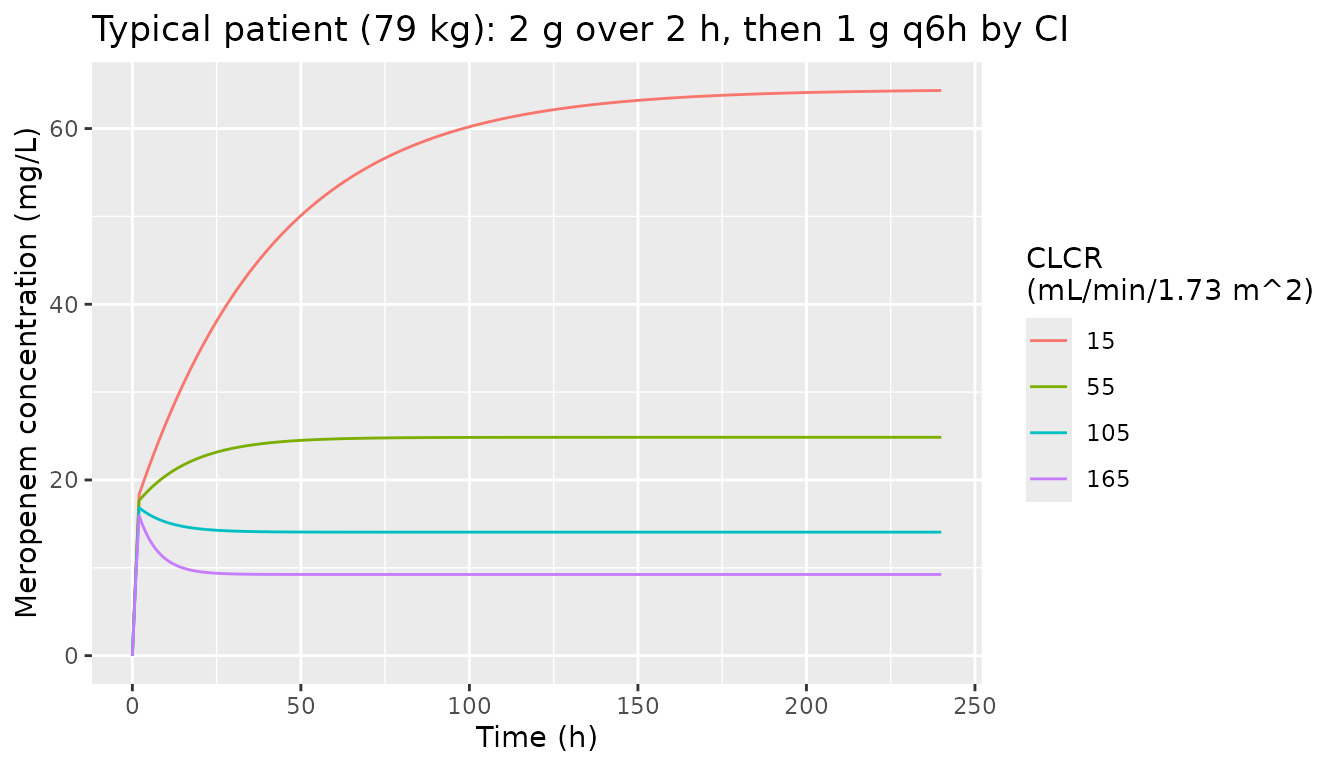
At the end of a long infusion the concentration approaches
rate / CL. This closed form depends only on clearance, so
it checks the clearance equation and its units directly.
css_check <- sim_typ |>
  filter(time == 240) |>
  mutate(
    cl_typ = 1.040 + 0.103 * CRCL,
    v_typ = 7.343 * 79^0.612,
    # Remaining non-steady-state fraction of the constant-rate input at 240 h
    # plus the leftover of the 2 g loading dose, both from the one-compartment
    # closed form.
    k = cl_typ / v_typ,
    css_expected = rate_1g_q6h / cl_typ * (1 - exp(-k * 238)) +
      2000 / cl_typ * (exp(-k * 238) - exp(-k * 240)) / 2,
    rel_err = Cc / css_expected - 1
  )
knitr::kable(
  css_check |>
    select(CRCL, cl_typ, css_expected, Cc, rel_err) |>
    dplyr::rename(
      "CLCR" = CRCL, "Typical CL (L/h)" = cl_typ,
      "Closed form at 240 h (mg/L)" = css_expected, "Simulated (mg/L)" = Cc,
      "Relative error" = rel_err
    ),
  digits = c(0, 2, 3, 3, 8)
)| CLCR | Typical CL (L/h) | Closed form at 240 h (mg/L) | Simulated (mg/L) | Relative error |
|---|---|---|---|---|
| 15 | 2.58 | 64.332 | 64.332 | 0 |
| 55 | 6.70 | 24.857 | 24.857 | 0 |
| 105 | 11.86 | 14.059 | 14.059 | 0 |
| 165 | 18.03 | 9.241 | 9.241 | 0 |
PKNCA validation
The paper reports no NCA. As a structural check, a single 2 g dose
infused over 2 h is given to typical patients at four CLCR values.
AUC0-inf must equal Dose / CL and the terminal
half-life must equal log(2) * V / CL.
ev_sd <- bind_rows(lapply(seq_along(crcl_levels), function(i) {
  bind_rows(
    data.frame(id = i, time = 0, amt = 2000, rate = 1000, evid = 1L, cmt = "central"),
    data.frame(id = i, time = c(0, 0.5, 1, 2, 3, 4, 6, 8, 12, seq(24, 480, by = 24)),
               amt = NA_real_, rate = NA_real_, evid = 0L, cmt = "central")
  ) |>
    mutate(CRCL = crcl_levels[i], WT = 79, treatment = paste0("CLCR ", crcl_levels[i]))
})) |>
  arrange(id, time, desc(evid))

sim_sd <- rxode2::rxSolve(mod_typ, ev_sd, returnType = "data.frame",
                          rtol = 1e-10, atol = 1e-12, maxsteps = 1e6) |>
  select(id, time, Cc) |>
  left_join(distinct(ev_sd, id, CRCL, treatment), by = "id")
#> ℹ omega/sigma items treated as zero: 'etalcl_nonren', 'etae_crcl_cl_renal', 'etalvc', 'etae_wt_vc'
#> Warning: multi-subject simulation without without 'omega'

# At high CLCR the 480 h grid runs dozens of half-lives past the dose, where
# the ODE solution is integrator noise around zero. Assert the undershoot is
# noise, floor it, and drop the numerically-zero tail after the peak so the
# log-down trapezoid and the half-life fit see only real decay.
stopifnot(all(sim_sd$Cc >= -1e-6 * max(sim_sd$Cc, na.rm = TRUE), na.rm = TRUE))
conc_sd <- sim_sd |>
  filter(!is.na(Cc)) |>
  mutate(Cc = pmax(Cc, 0)) |>
  group_by(id) |>
  filter(time <= time[which.max(Cc)] | Cc >= 1e-6 * max(Cc)) |>
  ungroup() |>
  select(id, time, Cc, treatment)
dose_sd <- ev_sd |>
  filter(evid == 1) |>
  select(id, time, amt, treatment)

o_conc <- PKNCA::PKNCAconc(conc_sd, Cc ~ time | treatment + id)
o_dose <- PKNCA::PKNCAdose(dose_sd, amt ~ time | treatment + id)
intervals <- data.frame(start = 0, end = Inf, cmax = TRUE, tmax = TRUE,
                        aucinf.obs = TRUE, half.life = TRUE)
nca <- PKNCA::pk.nca(PKNCA::PKNCAdata(o_conc, o_dose, intervals = intervals))

nca_wide <- as.data.frame(nca$result) |>
  filter(PPTESTCD %in% c("cmax", "aucinf.obs", "half.life")) |>
  select(treatment, PPTESTCD, PPORRES) |>
  pivot_wider(names_from = PPTESTCD, values_from = PPORRES) |>
  mutate(
    CRCL = as.numeric(sub("CLCR ", "", treatment)),
    cl_typ = 1.040 + 0.103 * CRCL,
    v_typ = 7.343 * 79^0.612,
    auc_expected = 2000 / cl_typ,
    thalf_expected = log(2) * v_typ / cl_typ
  ) |>
  arrange(CRCL)

knitr::kable(
  nca_wide |>
    select(treatment, cmax, aucinf.obs, auc_expected, half.life, thalf_expected) |>
    dplyr::rename(
      "Arm" = treatment, "Cmax (mg/L)" = cmax, "AUC0-inf PKNCA (mg*h/L)" = aucinf.obs,
      "Dose/CL (mg*h/L)" = auc_expected, "t1/2 PKNCA (h)" = half.life,
      "log(2)*V/CL (h)" = thalf_expected
    ),
  digits = 2
)| Arm | Cmax (mg/L) | AUC0-inf PKNCA (mg*h/L) | Dose/CL (mg*h/L) | t1/2 PKNCA (h) | log(2)*V/CL (h) |
|---|---|---|---|---|---|
| CLCR 15 | 18.34 | 773.67 | 773.69 | 28.55 | 28.55 |
| CLCR 55 | 17.65 | 298.23 | 298.28 | 11.01 | 11.01 |
| CLCR 105 | 16.84 | 168.61 | 168.71 | 6.23 | 6.23 |
| CLCR 165 | 15.93 | 110.76 | 110.90 | 4.09 | 4.09 |
# The trapezoidal AUC on this grid and the log-linear half-life fit carry a
# little numerical error; 2% is far below the tens-of-percent shift a
# mis-transcribed theta would cause.
stopifnot(
  max(abs(nca_wide$aucinf.obs / nca_wide$auc_expected - 1)) < 0.02,
  max(abs(nca_wide$half.life / nca_wide$thalf_expected - 1)) < 0.02
)
Replicating Figure 5: probability of target attainment
Section 3.4 simulated 1,000 patients per CLCR class (0-29, 30-79, 80-129 and 130-200 mL/min/1.73 m^2, CLCR uniform within each class) and computed the probability that the concentration at 72 h reached at least 4.63 x MIC. It tested several CI regimens. Here 200 virtual patients are drawn per CLCR class, and every regimen in the class is given to the same patients. The random effects are drawn in base R with a fixed seed and passed to the typical-value model as data, so the cohort is identical on every machine. Body weight, which the paper does not describe for the simulation, is drawn log-normally around the cohort median of 79 kg (log-scale SD 0.198, from the Table 1 IQR). Weights outside the observed 50-160 kg range are redrawn, not clamped. Each regimen starts with the institutional 2 g loading dose over 2 h, followed by the regimen’s continuous infusion. The loading dose is an assumption; see below.
set.seed(20211208)
n_per_class <- 200
crcl_classes <- data.frame(
  panel = c("CLCR 0-29", "CLCR 30-79", "CLCR 80-129", "CLCR 130-200"),
  lo = c(0, 30, 80, 130), hi = c(29, 79, 129, 200)
)
draw_wt <- function(n) {
  wt <- exp(rnorm(n, log(79), 0.198))
  bad <- wt < 50 | wt > 160
  while (any(bad)) {
    wt[bad] <- exp(rnorm(sum(bad), log(79), 0.198))
    bad <- wt < 50 | wt > 160
  }
  wt
}
omega <- c(etalcl_nonren = 0.465711, etae_crcl_cl_renal = 0.362263,
           etalvc = 0.198235, etae_wt_vc = 0.299975)
cohort <- bind_rows(lapply(seq_len(nrow(crcl_classes)), function(i) {
  data.frame(
    panel = crcl_classes$panel[i],
    CRCL = runif(n_per_class, crcl_classes$lo[i], crcl_classes$hi[i]),
    WT = draw_wt(n_per_class),
    etalcl_nonren = rnorm(n_per_class, 0, sqrt(omega[["etalcl_nonren"]])),
    etae_crcl_cl_renal = rnorm(n_per_class, 0, sqrt(omega[["etae_crcl_cl_renal"]])),
    etalvc = rnorm(n_per_class, 0, sqrt(omega[["etalvc"]])),
    etae_wt_vc = rnorm(n_per_class, 0, sqrt(omega[["etae_wt_vc"]]))
  )
})) |>
  mutate(subj = row_number())
# Individual volumes implied by the drawn random effects (used in the text).
cohort_v <- with(cohort, 7.343 * exp(etalvc) * WT^(0.612 * exp(etae_wt_vc)))

regimens <- data.frame(
  regimen = c("0.25g q6h CI", "0.5g q6h CI", "1g q8h CI", "1g q6h CI",
              "1.25g q6h CI", "1.5g q6h CI", "2g q6h CI", "2.5g q6h CI"),
  rate = c(250 / 6, 500 / 6, 1000 / 8, 1000 / 6, 1250 / 6, 1500 / 6, 2000 / 6, 2500 / 6)
)
# Figure 5 shows 0.25-1.5 g in the three lower classes and 1-2.5 g in the top class.
panel_regimens <- bind_rows(
  expand.grid(panel = crcl_classes$panel[1:3], regimen = regimens$regimen[1:6],
              stringsAsFactors = FALSE),
  expand.grid(panel = crcl_classes$panel[4], regimen = regimens$regimen[3:8],
              stringsAsFactors = FALSE)
) |>
  left_join(regimens, by = "regimen")

css72 <- function(model, loading_dose) {
  ev <- panel_regimens |>
    inner_join(cohort, by = "panel", relationship = "many-to-many") |>
    mutate(id = row_number())
  doses <- bind_rows(
    if (loading_dose > 0) {
      transmute(ev, id, time = 0, amt = loading_dose, rate = loading_dose / 2, evid = 1L)
    },
    transmute(ev, id, time = if (loading_dose > 0) 2 else 0,
              amt = rate * 100, rate = rate, evid = 1L)
  )
  obs <- transmute(ev, id, time = 72, amt = NA_real_, rate = NA_real_, evid = 0L)
  events <- bind_rows(doses, obs) |>
    mutate(cmt = "central") |>
    left_join(select(ev, id, CRCL, WT, starts_with("eta")), by = "id") |>
    arrange(id, time, desc(evid))
  sim <- rxode2::rxSolve(model, events, returnType = "data.frame", maxsteps = 1e6)
  stopifnot(nrow(sim) == nrow(ev), !anyNA(sim$Cc))
  ev |>
    select(id, panel, regimen, rate) |>
    mutate(Css72 = sim$Cc[match(id, sim$id)])
}
pta_ld <- css72(mod_typ, loading_dose = 2000)
#> ℹ omega/sigma items treated as zero: 'etalcl_nonren', 'etae_crcl_cl_renal', 'etalvc', 'etae_wt_vc'
#> Warning: multi-subject simulation without without 'omega'
mic_grid <- 2^seq(log2(0.125), log2(32), length.out = 97)
pta_curves <- pta_ld |>
  group_by(panel, regimen) |>
  reframe(MIC = mic_grid,
          PTA = sapply(mic_grid, function(m) 100 * mean(Css72 / m >= 4.63))) |>
  mutate(panel = factor(panel, levels = crcl_classes$panel),
         regimen = factor(regimen, levels = regimens$regimen))

ggplot(pta_curves, aes(MIC, PTA, colour = regimen)) +
  geom_line() +
  geom_hline(yintercept = 90, linetype = "dotted") +
  scale_x_continuous(trans = "log2", breaks = 2^(-3:5), labels = c(0.125, 0.25, 0.5, 1, 2, 4, 8, 16, 32)) +
  facet_wrap(~panel) +
  labs(x = "MIC (mg/L)", y = "PTA (%)", colour = NULL,
       title = "Replicates Figure 5 of Cojutti 2021 (Css/MIC >= 4.63 at 72 h)")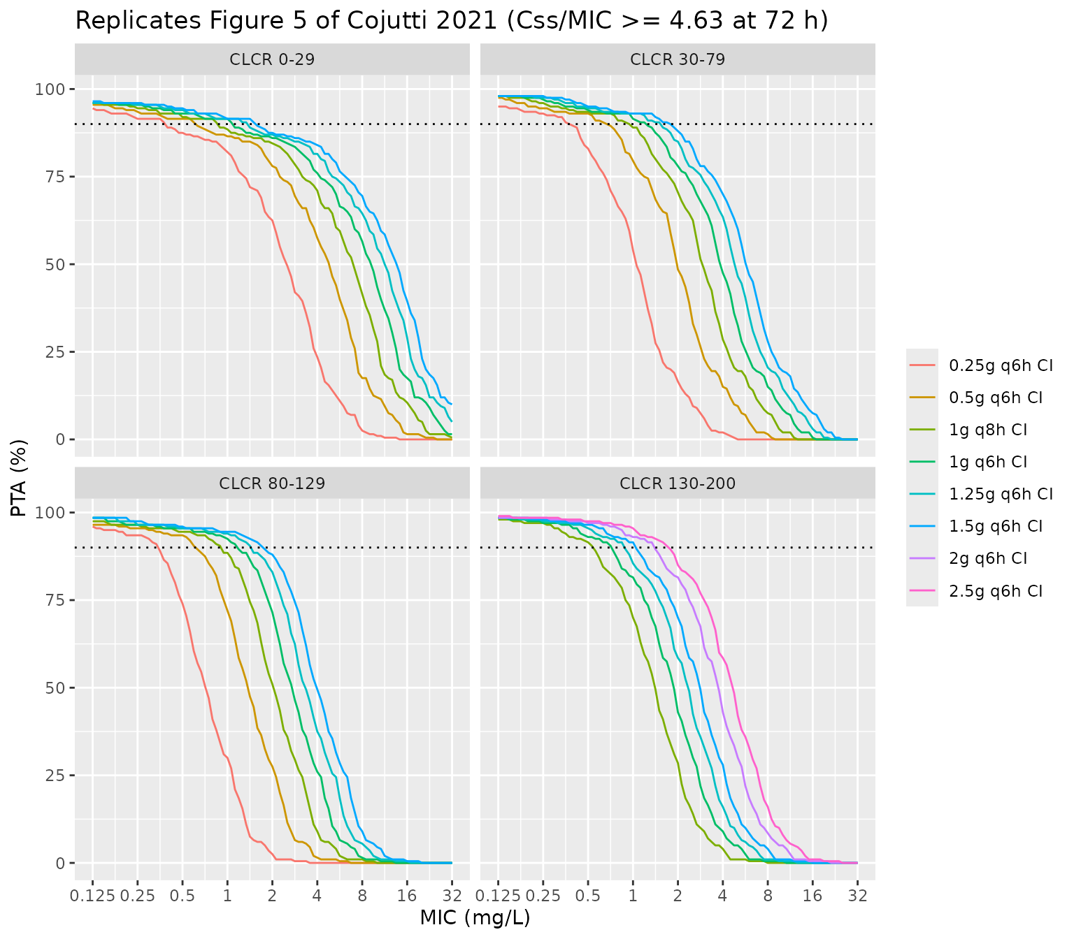
The paper’s curves were digitized from Figure 5. The digitization located the plot’s axis ticks and traced each curve by colour. For each curve it recorded the MIC at which PTA crosses 50%, which equals the median Css divided by 4.63, and the MIC at which PTA crosses 90%. The same quantities are computed from the simulation.
fig5 <- tribble(
  ~panel,         ~regimen,       ~mic50_paper, ~mic90_paper,
  "CLCR 0-29",    "0.25g q6h CI",  2.771, 1.043,
  "CLCR 0-29",    "0.5g q6h CI",   5.057, 1.747,
  "CLCR 0-29",    "1g q8h CI",     7.282, 2.511,
  "CLCR 0-29",    "1g q6h CI",     9.671, 3.177,
  "CLCR 0-29",    "1.25g q6h CI", 11.707, 3.775,
  "CLCR 0-29",    "1.5g q6h CI",  14.019, 4.590,
  "CLCR 30-79",   "0.25g q6h CI",  1.235, 0.534,
  "CLCR 30-79",   "0.5g q6h CI",   2.368, 1.026,
  "CLCR 30-79",   "1g q8h CI",     3.321, 1.509,
  "CLCR 30-79",   "1g q6h CI",     4.596, 1.969,
  "CLCR 30-79",   "1.25g q6h CI",  5.630, 2.395,
  "CLCR 30-79",   "1.5g q6h CI",   6.525, 2.916,
  "CLCR 80-129",  "0.25g q6h CI",  0.733, 0.318,
  "CLCR 80-129",  "0.5g q6h CI",   1.413, 0.628,
  "CLCR 80-129",  "1g q8h CI",     2.042, 0.955,
  "CLCR 80-129",  "1g q6h CI",     2.794, 1.246,
  "CLCR 80-129",  "1.25g q6h CI",  3.373, 1.590,
  "CLCR 80-129",  "1.5g q6h CI",   4.048, 1.894,
  "CLCR 130-200", "1g q8h CI",     1.431, 0.633,
  "CLCR 130-200", "1g q6h CI",     1.836, 0.874,
  "CLCR 130-200", "1.25g q6h CI",  2.355, 1.070,
  "CLCR 130-200", "1.5g q6h CI",   2.825, 1.256,
  "CLCR 130-200", "2g q6h CI",     3.656, 1.750,
  "CLCR 130-200", "2.5g q6h CI",   4.713, 2.141
)
sim_mic <- pta_ld |>
  group_by(panel, regimen, rate) |>
  summarise(mic50_sim = median(Css72) / 4.63,
            mic90_sim = unname(quantile(Css72, 0.10)) / 4.63, .groups = "drop")
cmp <- fig5 |>
  left_join(sim_mic, by = c("panel", "regimen")) |>
  mutate(pct50 = 100 * (mic50_sim / mic50_paper - 1),
         pct90 = 100 * (mic90_sim / mic90_paper - 1))
stopifnot(nrow(cmp) == 24L, !anyNA(cmp$mic50_sim))
knitr::kable(
  cmp |>
    select(panel, regimen, mic50_paper, mic50_sim, pct50, mic90_paper, mic90_sim, pct90) |>
    dplyr::rename(
      "CLCR class" = panel, "Regimen" = regimen,
      "MIC at 50% PTA, Figure 5" = mic50_paper, "MIC at 50% PTA, simulated" = mic50_sim,
      "Diff 50% (%)" = pct50,
      "MIC at 90% PTA, Figure 5" = mic90_paper, "MIC at 90% PTA, simulated" = mic90_sim,
      "Diff 90% (%)" = pct90
    ),
  digits = 2
)| CLCR class | Regimen | MIC at 50% PTA, Figure 5 | MIC at 50% PTA, simulated | Diff 50% (%) | MIC at 90% PTA, Figure 5 | MIC at 90% PTA, simulated | Diff 90% (%) |
|---|---|---|---|---|---|---|---|
| CLCR 0-29 | 0.25g q6h CI | 2.77 | 2.50 | -9.93 | 1.04 | 0.39 | -62.45 |
| CLCR 0-29 | 0.5g q6h CI | 5.06 | 4.79 | -5.22 | 1.75 | 0.63 | -63.98 |
| CLCR 0-29 | 1g q8h CI | 7.28 | 6.97 | -4.27 | 2.51 | 0.87 | -65.42 |
| CLCR 0-29 | 1g q6h CI | 9.67 | 9.09 | -5.96 | 3.18 | 1.11 | -65.18 |
| CLCR 0-29 | 1.25g q6h CI | 11.71 | 11.29 | -3.58 | 3.78 | 1.34 | -64.43 |
| CLCR 0-29 | 1.5g q6h CI | 14.02 | 13.48 | -3.84 | 4.59 | 1.58 | -65.59 |
| CLCR 30-79 | 0.25g q6h CI | 1.24 | 1.05 | -14.80 | 0.53 | 0.39 | -26.82 |
| CLCR 30-79 | 0.5g q6h CI | 2.37 | 1.97 | -16.93 | 1.03 | 0.69 | -33.18 |
| CLCR 30-79 | 1g q8h CI | 3.32 | 2.91 | -12.40 | 1.51 | 0.96 | -36.63 |
| CLCR 30-79 | 1g q6h CI | 4.60 | 3.87 | -15.90 | 1.97 | 1.23 | -37.53 |
| CLCR 30-79 | 1.25g q6h CI | 5.63 | 4.77 | -15.19 | 2.40 | 1.50 | -37.19 |
| CLCR 30-79 | 1.5g q6h CI | 6.53 | 5.69 | -12.81 | 2.92 | 1.80 | -38.19 |
| CLCR 80-129 | 0.25g q6h CI | 0.73 | 0.71 | -2.89 | 0.32 | 0.34 | 7.75 |
| CLCR 80-129 | 0.5g q6h CI | 1.41 | 1.36 | -3.74 | 0.63 | 0.60 | -5.00 |
| CLCR 80-129 | 1g q8h CI | 2.04 | 2.02 | -1.11 | 0.96 | 0.89 | -6.32 |
| CLCR 80-129 | 1g q6h CI | 2.79 | 2.68 | -3.94 | 1.25 | 1.16 | -6.75 |
| CLCR 80-129 | 1.25g q6h CI | 3.37 | 3.34 | -0.96 | 1.59 | 1.43 | -10.23 |
| CLCR 80-129 | 1.5g q6h CI | 4.05 | 3.98 | -1.70 | 1.89 | 1.70 | -10.20 |
| CLCR 130-200 | 1g q8h CI | 1.43 | 1.40 | -1.85 | 0.63 | 0.55 | -12.77 |
| CLCR 130-200 | 1g q6h CI | 1.84 | 1.86 | 1.54 | 0.87 | 0.71 | -18.32 |
| CLCR 130-200 | 1.25g q6h CI | 2.36 | 2.32 | -1.31 | 1.07 | 0.88 | -18.12 |
| CLCR 130-200 | 1.5g q6h CI | 2.83 | 2.78 | -1.43 | 1.26 | 1.04 | -16.82 |
| CLCR 130-200 | 2g q6h CI | 3.66 | 3.71 | 1.55 | 1.75 | 1.39 | -20.42 |
| CLCR 130-200 | 2.5g q6h CI | 4.71 | 4.63 | -1.75 | 2.14 | 1.74 | -18.70 |
# The median Css of 200 draws has a sampling SE of about 1.25 * 0.85 / sqrt(200)
# = 7.5% (log-scale SD of Css ~0.85). The draw is fixed by the base-R seed. A
# mis-transcribed theta, dose or unit shifts every cell by tens of percent.
stopifnot(
  abs(median(cmp$pct50)) < 10,
  quantile(abs(cmp$pct50), 0.9) < 20
)
The centre of every curve is reproduced: the median difference in the MIC at 50% PTA is -3.8% across the 24 curves. The simulated MIC at 90% PTA is systematically lower than the paper’s, by a median of -24% overall. The gap is largest in the CLCR 0-29 class (median -65%). The simulated left tail of Css is heavier than the paper’s because of how the NPAG result has to be encoded (see Assumptions and deviations). The gap is widest at low CLCR because there a patient drawn with a very large volume is still far from steady state at 72 h.
The loading dose, and why the volume is large
Section 2.5 does not say whether the simulated regimens began with a loading dose. For a linear model the concentration at 72 h is exactly proportional to the infusion rate if there is no loading dose, and so is the MIC at 50% PTA. Figure 5 is not proportional in the lowest CLCR class. The paper’s MIC at 50% PTA per unit infusion rate is 18.6% higher for 0.25 g q6h than for 1.5 g q6h. This is the signature of a fixed loading dose that has not yet washed out at 72 h. A loading dose can only persist that long if the half-life is long, which requires a large volume.
The table repeats the lowest-CLCR panel in three ways: as above; without a loading dose; and with the loading dose but the volume replaced by 20 L. 20 L is the paper’s median individual (Bayesian posterior) V.
mod_v20 <- mod_typ |>
  rxode2::ini(lvc = log(20), e_wt_vc = 0)
#> ℹ change initial estimate of `lvc` to `2.99573227355399`
#> ℹ change initial estimate of `e_wt_vc` to `0`
pta_nold <- css72(mod_typ, loading_dose = 0)
#> ℹ omega/sigma items treated as zero: 'etalcl_nonren', 'etae_crcl_cl_renal', 'etalvc', 'etae_wt_vc'
#> Warning: multi-subject simulation without without 'omega'
pta_v20 <- css72(mod_v20, loading_dose = 2000)
#> ℹ omega/sigma items treated as zero: 'etalcl_nonren', 'etae_crcl_cl_renal', 'etalvc', 'etae_wt_vc'
#> Warning: multi-subject simulation without without 'omega'

prop_ratio <- function(d, panel_name = "CLCR 0-29") {
  m <- d |>
    filter(panel == panel_name) |>
    group_by(regimen, rate) |>
    summarise(mic50 = median(Css72) / 4.63, .groups = "drop")
  lo <- m[m$regimen == "0.25g q6h CI", ]
  hi <- m[m$regimen == "1.5g q6h CI", ]
  (lo$mic50 / lo$rate) / (hi$mic50 / hi$rate)
}
ratio_tab <- data.frame(
  scenario = c("Figure 5 (digitized)", "Model, 2 g loading dose (as simulated above)",
               "Model, no loading dose", "2 g loading dose, V fixed at 20 L"),
  ratio = c((2.771 / (250 / 6)) / (14.019 / (1500 / 6)), prop_ratio(pta_ld),
            prop_ratio(pta_nold), prop_ratio(pta_v20))
)
knitr::kable(
  ratio_tab |>
    dplyr::rename("Scenario" = scenario,
                  "Rate-normalized MIC50, 0.25 g vs 1.5 g q6h (CLCR 0-29)" = ratio),
  digits = 3
)| Scenario | Rate-normalized MIC50, 0.25 g vs 1.5 g q6h (CLCR 0-29) |
|---|---|
| Figure 5 (digitized) | 1.186 |
| Model, 2 g loading dose (as simulated above) | 1.111 |
| Model, no loading dose | 1.000 |
| 2 g loading dose, V fixed at 20 L | 1.000 |
# Without a loading dose the ratio is exactly 1 (linearity). With V = 20 L the
# loading dose has washed out by 72 h, so the ratio is also 1. The printed V
# with the loading dose reproduces the paper's departure from proportionality.
stopifnot(
  abs(ratio_tab$ratio[3] - 1) < 1e-3,
  abs(ratio_tab$ratio[4] - 1) < 0.01,
  ratio_tab$ratio[2] > 1.08
)
Assumptions and deviations
-
Volume of distribution. Evaluated at the Table 4
means,
V = 7.343 * BW^0.612gives 106 L at 79 kg. The Results report a median individual (Bayesian posterior) V of 20.0 L (IQR 17.16-23.59). The two are not contradictory under a non-parametric fit. The four thetas are means of marginal support-point distributions, the exponent itself is random (CV 59%), and V is a strongly non-linear function of it. The posterior values also shrink toward the data, and steady-state CI data carry little information on V. The model encodes the equation and values exactly as printed. The loading-dose analysis above shows that Figure 5 reproduces only with the large printed volume; a 20 L volume removes the departure from dose proportionality that the figure shows. Clearance, not volume, sets every steady-state concentration. - Loading dose in the simulations. Section 2.5 does not state one. The institutional 2 g over 2 h (Section 2.1) was assumed because it reproduces Figure 5, and the alternative without a loading dose does not.
-
NPAG to log-normal. Table 4 gives only the mean and
CV% of each marginal distribution. The means are used as typical
(median) values of independent log-normal random effects, with
omega^2 = log(CV^2 + 1). This is the convention used by the other Pmetrics models in the library. The NPAG joint density, including the intercept-slope and theta3-theta4 correlations, is not published. The independent log-normal tails are wider than the bounded NPAG support. This is why the simulated MIC at 90% PTA falls below Figure 5, while the median is reproduced. The volume tail is the extreme case. With independent random effects on theta3 and on the exponent, 14% of the simulated Figure 5 cohort has a volume above 1,000 L (median 110 L). The paper’s posterior V IQR of 17-24 L suggests that theta3 and theta4 are strongly negatively correlated in the NPAG joint density. Stochastic simulations from this model therefore understate the lower percentiles of concentration before steady state, most of all in renal impairment. Typical-value and steady-state results are unaffected. -
Random effect on an exponent. Theta4 is a random
parameter in the NPAG fit, so its CV is carried as
etae_wt_vc, a log-normal multiplier on the exponent. This keeps the exponent positive, as the paper describes it (‘the positive exponent estimate’). -
Residual error. Section 2.4 gives the assay
polynomial
0.0798 + 0.0927 * C(C2 = C3 = 0) and ‘a gamma model (gamma = 2)’. Pmetrics multiplies the polynomial SD by gamma, which gives an additive SD of 0.1596 mg/L plus a proportional SD of 0.1854, summed on the SD scale (combined1()). The text does not say whether 2 is the final estimate of gamma or its starting value; it is taken as printed. - Body weight in the simulations. The paper does not describe the weight distribution used in its Monte Carlo simulation. A log-normal around 79 kg matching the Table 1 IQR, truncated by redrawing to 50-160 kg, was used.
- Figure 5 digitization. Performed by the maintainers from the published figure image by colour-tracing each curve against the axis ticks. The reading uncertainty is small next to the 200-subject sampling error.
- Clinical-outcome analysis not encoded. The CART and logistic-regression analysis of clinical cure against Css/MIC >= 4.63 (Section 3.2, Table 3) is a threshold classification, not a dynamic model. The 4.63 threshold is used above only as the PTA target.