Mycophenolic acid (Fromage 2025)
Source:vignettes/articles/Fromage_2025_mycophenolic_acid.Rmd
Fromage_2025_mycophenolic_acid.RmdModel and source
- Citation: Fromage Y, Sayadi H, Koloskoff K, Marquet P, Labriffe M, Monchaud C, Woillard JB. Killing several birds with one stone: A multi-indication population pharmacokinetic model and Bayesian estimator for enteric-coated mycophenolate sodium. Br J Clin Pharmacol. 2025;91(5):1396-1408. doi:10.1111/bcp.16374.
- Description: One-compartment population PK model for mycophenolic acid (MPA) after oral enteric-coated mycophenolate sodium (EC-MPS, Myfortic) in a multi-indication cohort of solid-organ transplant, haematopoietic cell transplant and autoimmune-disease patients (Fromage 2025), with double-gamma absorption describing the characteristic double concentration peak, first-order elimination, a steady-state trough offset, and an indication effect on the second gamma rate constant. Evaluated in the closed form published by the authors (Monolix fitted the analytic solution), so the model is a steady-state single-dosing-interval model.
- Article: https://doi.org/10.1111/bcp.16374
Mycophenolic acid (MPA) is the active moiety of enteric-coated mycophenolate sodium (EC-MPS, Myfortic). Fromage 2025 is the first population PK model for EC-MPS built across multiple indications rather than in renal transplantation alone, and the first to apply a double-gamma absorption model to this formulation. The enteric coating delays release into the small intestine and produces the erratic, frequently double-peaked absorption profiles that motivate the gamma mixture.
Population
The model was built from retrospective real-world therapeutic-drug-monitoring data extracted from the ISBA / ABIS 3.0 Bayesian dose-adaptation platform at Limoges University Hospital: 153 PK profiles comprising 863 MPA concentrations from 129 patients (Section 3.1). All patients received Myfortic. Indications span renal, hepatic, cardiac and pulmonary transplantation, bone marrow / haematopoietic cell transplantation, and autoimmune disease (systemic lupus erythematosus, lupus nephritis, nephrotic syndrome): 116 patients with solid-organ or haematopoietic cell transplantation and 13 with autoimmune disease. Median age was 45 years (range 6 to 80), and 20 of 127 patients were paediatric (< 18 years). EC-MPS doses ranged from 180 to 1440 mg per intake with a median of 360 mg. Sampling was sparse and irregular (3 to 11 samples per profile, median 5). Baseline characteristics are given in Table 1.
Body weight, serum albumin and creatinine clearance – the covariates most often reported to influence MPA clearance – were not available in the ISBA extraction, which the authors identify as a limitation (Section 4).
The same information is available programmatically via the model’s
population metadata
(readModelDb("Fromage_2025_mycophenolic_acid")()$population).
Model structure
A one-compartment model with first-order elimination and a double-gamma absorption input best described the data (Section 3.2.1). The absorption rate is a two-component gamma mixture (Section 2.2.1),
and the authors give the resulting plasma concentration in closed form,
where is the regularised lower incomplete gamma function, is the steady-state trough concentration, is the disposition coefficient and the disposition rate constant.
That closed form is what Monolix fitted, and it is what the packaged
model evaluates, using rxode2’s gammap(a, z) for
.
Two consequences are worth stating up front:
- The gamma components are stored in the canonical transit
parameterisation
(ntr, mtt)with and , somttis exactly the paper’s mean absorption time MAT. - Because
tad()andpodo()refer to the most recent dose, the model describes one steady-state dosing interval and does not accumulate across doses. This matches the authors’ framing, in which is the trough carried in from previous doses.
Source trace
The per-parameter origin is recorded as an in-file comment next to
each ini() entry in
inst/modeldb/specificDrugs/Fromage_2025_mycophenolic_acid.R.
The table below collects them in one place for review.
| Equation / parameter | Value | Source location |
|---|---|---|
Absorption input rate Va(t) (gamma mixture) |
n/a | Section 2.2.1, first two display equations |
Closed-form C(t)
|
n/a | Section 2.2.1, third display equation |
MATi = ai / bi, V/F = 100 / FAIV,
CL/F = Dose / AUC
|
n/a | Section 2.2.1, final three display equations |
Categorical covariate model on log(b2)
|
n/a | Section 2.2.2, categorical-covariate equation and the
log(b2) IIV equation |
lntr1 (a1 = 1280.97) |
1279.97 | Table 2, a1 (RSE 0.25%) |
lmtt1 (a1/b1) |
3.061 h | Table 2, a1 = 1280.97 and b1 = 418.42
1/h |
lntr2 (a2 = 395.34) |
394.34 | Table 2, a2 (RSE 2.30%) |
lmtt2 (a2/b2) |
4.131 h | Table 2, a2 = 395.34 and b2 = 95.69
1/h |
lfdepot (r) |
0.79 | Table 2, r (RSE 2.14%) |
lvc (100/FAIV) |
12.71 L | Table 2, FAIV = 7.87 mg/L (RSE 3.35%) |
lkel (lambda) |
1.81 1/h | Table 2, lambda (RSE 7.48%) |
lrbase (C0) |
2.21 mg/L | Table 2, C0 (RSE 6.50%) |
e_tx_heart_lung_hct_mtt2 |
-0.59 | Table 2,
beta_b2_cardiac, pulmonary, bone marrow transplantations =
+0.59 on log(b2) (RSE 47.1%); sign inverts on
log(MAT2)
|
e_dis_autoimmune_mtt2 |
+0.17 | Table 2, beta_b2_autoimmune diseases = -0.17 on
log(b2) (RSE 188%); sign inverts on
log(MAT2)
|
etalmtt1 |
0.8464 | Table 2, IIV b1 = 0.92 SD (RSE 44.9%); variance =
SD^2 |
etalmtt2 |
0.2704 | Table 2, IIV b2 = 0.52 SD (RSE 16.1%) |
etalvc |
0.0144 | Table 2, IIV FAIV = 0.12 SD (RSE 11.0%) |
etalkel |
0.1936 | Table 2, IIV lambda = 0.44 SD (RSE 14.2%) |
etalrbase |
0.2401 | Table 2, IIV C0 = 0.49 SD (RSE 10.8%) |
addSd |
1.38 mg/L | Table 2, residual additive error sigma (RSE 3.47%) |
Table 2’s footnote states that “IIV and IOV are expressed as SD”,
which is why each eta variance above is the reported value
squared.
Gate 1: the packaged model reproduces the published closed form
The strongest available structural check is to evaluate the paper’s
printed equation independently – in plain R, with
stats::pgamma() supplying
– and compare it against a solve of the packaged model. Nothing is
fitted or tuned here; agreement to numerical precision means the ODE
wiring, the (ntr, mtt) to
mapping, the FAIV to vc conversion, the
bioavailability split and the trough offset are all correct
simultaneously.
mod <- readModelDb("Fromage_2025_mycophenolic_acid")
mod_typ <- rxode2::zeroRe(rxode2::rxode(mod))
#> ℹ parameter labels from comments will be replaced by 'label()'

# Table 2 values, transcribed once for the independent evaluation.
p <- list(C0 = 2.21, a1 = 1280.97, b1 = 418.42, a2 = 395.34, b2 = 95.69,
          FAIV = 7.87, lambda = 1.81, r = 0.79)
p$vc <- 100 / p$FAIV

published_closed_form <- function(t, dose, b2 = p$b2) {
  arm1 <- p$r * (p$b1 / (p$b1 - p$lambda))^p$a1 *
    stats::pgamma((p$b1 - p$lambda) * t, shape = p$a1)
  arm2 <- (1 - p$r) * (b2 / (b2 - p$lambda))^p$a2 *
    stats::pgamma((b2 - p$lambda) * t, shape = p$a2)
  p$C0 + (dose / p$vc) * (arm1 + arm2) * exp(-p$lambda * t)
}

# Reference indication group (renal / hepatic): all indicators zero.
ref_cov <- list(TX_HEART = 0, TX_LUNG = 0, TX_HCT = 0, DIS_AUTOIMMUNE = 0)

make_events <- function(dose, cov, times) {
  ev <- as.data.frame(rxode2::et(amt = dose, cmt = "depot") |> rxode2::et(times))
  for (nm in names(cov)) ev[[nm]] <- cov[[nm]]
  ev
}

times_fine <- seq(0, 12, by = 0.01)
sim_typ <- rxode2::rxSolve(mod_typ, make_events(720, ref_cov, times_fine))
#> ℹ omega/sigma items treated as zero: 'etalmtt1', 'etalmtt2', 'etalvc', 'etalkel', 'etalrbase'

err <- max(abs(sim_typ$Cc - published_closed_form(sim_typ$time, 720)))
cat(sprintf("max |packaged - published closed form| = %.3e mg/L\n", err))
#> max |packaged - published closed form| = 6.963e-13 mg/L
stopifnot(err < 1e-8)
The agreement is at the level of double-precision round-off, so the packaged model is the published equation rather than an approximation of it.
Gate 2: derived-parameter identities
The paper prints three derived-parameter relations (Section 2.2.1) and quotes two of the resulting values in the Abstract. Each is checked below.
mat1 <- p$a1 / p$b1
mat2 <- p$a2 / p$b2
vdf  <- 100 / p$FAIV

identities <- tibble::tibble(
  Quantity = c("V/F = 100/FAIV (L)", "MAT1 = a1/b1 (h)", "MAT2 = a2/b2 (h)",
               "C(0) = C0, the steady-state trough (mg/L)"),
  Recovered = c(vdf, mat1, mat2, sim_typ$Cc[sim_typ$time == 0]),
  Published = c(12.60, NA_real_, 4.09, 2.21),
  `Source` = c("Abstract (Vd/F = 12.60 L)", "not quoted separately",
               "Discussion (4.09 h; see Errata)", "Table 2 (C0)")
)
knitr::kable(identities, digits = 4,
caption = "Derived-parameter identities against the published values.")| Quantity | Recovered | Published | Source |
|---|---|---|---|
| V/F = 100/FAIV (L) | 12.7065 | 12.60 | Abstract (Vd/F = 12.60 L) |
| MAT1 = a1/b1 (h) | 3.0614 | NA | not quoted separately |
| MAT2 = a2/b2 (h) | 4.1315 | 4.09 | Discussion (4.09 h; see Errata) |
| C(0) = C0, the steady-state trough (mg/L) | 2.2100 | 2.21 | Table 2 (C0) |
# The trough identity is exact by construction and must hold.
stopifnot(abs(sim_typ$Cc[sim_typ$time == 0] - p$C0) < 1e-10)
# V/F must land within 1% of the Abstract's rounded 12.60 L.
stopifnot(abs(vdf - 12.60) / 12.60 < 0.01)
V/F recovers 12.71 L against the Abstract’s 12.60 L, a
0.9% difference attributable to rounding of FAIV to three
significant figures. The MAT2 discrepancy is a slip in the paper and is
analysed in the Errata below.
Gate 3: the indication covariate reproduces Table 2 and the Discussion
Fromage 2025 retained a single covariate: the three-level indication
grouping acting on the second gamma rate constant b2. The
Discussion quotes the resulting b2 values and mean
absorption times for all three groups, which makes this an unusually
well-specified check – the packaged model must reproduce six published
numbers from two estimated coefficients.
groups <- tibble::tribble(
  ~group,                              ~TX_HEART, ~TX_LUNG, ~TX_HCT, ~DIS_AUTOIMMUNE,
  "(i) renal / hepatic (reference)",           0,        0,       0,               0,
  "(ii) cardiac",                              1,        0,       0,               0,
  "(ii) pulmonary",                            0,        1,       0,               0,
  "(ii) haematopoietic cell",                  0,        0,       1,               0,
  "(iii) autoimmune disease",                  0,        0,       0,               1
)

recovered <- lapply(seq_len(nrow(groups)), function(i) {
  cov <- as.list(groups[i, c("TX_HEART", "TX_LUNG", "TX_HCT", "DIS_AUTOIMMUNE")])
  s <- rxode2::rxSolve(mod_typ, make_events(720, cov, times_fine))
  auc <- sum(diff(s$time) * (head(s$Cc, -1) + tail(s$Cc, -1)) / 2)
  tibble::tibble(group = groups$group[i], b2 = s$gb2[1], MAT2 = s$ga2[1] / s$gb2[1],
                 Cmax = max(s$Cc), Tmax = s$time[which.max(s$Cc)], AUC = auc)
}) |> dplyr::bind_rows()
#> ℹ omega/sigma items treated as zero: 'etalmtt1', 'etalmtt2', 'etalvc', 'etalkel', 'etalrbase'
#> ℹ omega/sigma items treated as zero: 'etalmtt1', 'etalmtt2', 'etalvc', 'etalkel', 'etalrbase'
#> ℹ omega/sigma items treated as zero: 'etalmtt1', 'etalmtt2', 'etalvc', 'etalkel', 'etalrbase'
#> ℹ omega/sigma items treated as zero: 'etalmtt1', 'etalmtt2', 'etalvc', 'etalkel', 'etalrbase'
#> ℹ omega/sigma items treated as zero: 'etalmtt1', 'etalmtt2', 'etalvc', 'etalkel', 'etalrbase'

recovered |>
  dplyr::mutate(
    `b2 published` = c(95.69, 172.62, 172.62, 172.62, 80.73),
    `MAT2 published` = c(4.09, 2.29, 2.29, 2.29, 4.90)
  ) |>
  dplyr::rename("Indication group" = group, "b2 (1/h)" = b2, "MAT2 (h)" = MAT2,
                "Cmax (mg/L)" = Cmax, "Tmax (h)" = Tmax, "AUC0-12 (mg*h/L)" = AUC) |>
  knitr::kable(digits = c(0, 2, 2, 3, 2, 2, 2, 2),
               caption = paste("Indication effect on the second gamma component.",
"Published b2 values and MAT2 are from the Discussion."))| Indication group | b2 (1/h) | MAT2 (h) | Cmax (mg/L) | Tmax (h) | AUC0-12 (mg*h/L) | b2 published | MAT2 published |
|---|---|---|---|---|---|---|---|
| (i) renal / hepatic (reference) | 95.69 | 4.13 | 34.864 | 3.20 | 57.83 | 95.69 | 4.09 |
| (ii) cardiac | 172.62 | 2.29 | 37.229 | 3.19 | 57.83 | 172.62 | 2.29 |
| (ii) pulmonary | 172.62 | 2.29 | 37.229 | 3.19 | 57.83 | 172.62 | 2.29 |
| (ii) haematopoietic cell | 172.62 | 2.29 | 37.229 | 3.19 | 57.83 | 172.62 | 2.29 |
| (iii) autoimmune disease | 80.73 | 4.90 | 34.864 | 3.20 | 57.83 | 80.73 | 4.90 |
# The three pooled group-(ii) indicators must give an identical b2, because the
# source estimates ONE effect for the pooled level.
grp2 <- recovered$b2[recovered$group %in%
                       c("(ii) cardiac", "(ii) pulmonary", "(ii) haematopoietic cell")]
stopifnot(length(grp2) == 3, diff(range(grp2)) < 1e-9)

# b2 must reproduce the Discussion's printed values to rounding.
stopifnot(max(abs(recovered$b2 - c(95.69, 172.62, 172.62, 172.62, 80.73))) < 0.01)

# AUC0-12 must be INVARIANT across indication groups: b2 shifts the timing of
# the second absorption peak but not the amount absorbed. This is a genuine
# falsifier -- had the covariate been wired onto vc or kel instead of mtt2,
# these AUCs would differ.
stopifnot(diff(range(recovered$AUC)) / mean(recovered$AUC) < 1e-6)
All five rows reproduce the published b2 exactly, the
three pooled group-(ii) indicators are numerically identical as they
must be, and AUC0-12 is invariant across groups – confirming the
covariate acts on absorption timing only. Group (ii) roughly
halves MAT2 (4.13 h to 2.29 h), which is the effect the authors
describe.
Virtual cohort
Original observed data are not publicly available. The cohort below uses the two most common EC-MPS strengths in the source (the median 360 mg intake and a 720 mg intake), 200 subjects per arm, with the reference renal / hepatic indication so the arms differ only in dose.
set.seed(20250421)

n_per_arm <- 200L
arm_doses <- c(`360 mg` = 360, `720 mg` = 720)

# Observation grid: 0.05 h over the interval, refined to 0.01 h across the
# absorption peak so Cmax and Tmax are resolved. The peak is genuinely sharp
# (component 1 has width ~sqrt(a1)/b1 = 0.086 h).
obs_times <- sort(unique(c(seq(0, 12, by = 0.05), seq(2.0, 4.5, by = 0.01))))

make_arm <- function(dose, label, id_offset) {
  ids <- id_offset + seq_len(n_per_arm)
  dosing <- tibble::tibble(id = ids, time = 0, amt = dose, evid = 1L,
                           cmt = "depot")
  obs <- tidyr::expand_grid(id = ids, time = obs_times) |>
    dplyr::mutate(amt = NA_real_, evid = 0L, cmt = "depot")
  dplyr::bind_rows(dosing, obs) |>
    dplyr::mutate(arm = label, TX_HEART = 0, TX_LUNG = 0, TX_HCT = 0,
                  DIS_AUTOIMMUNE = 0) |>
    dplyr::arrange(id, time, dplyr::desc(evid))
}

events <- dplyr::bind_rows(
  make_arm(arm_doses[["360 mg"]], "360 mg", id_offset = 0L),
  make_arm(arm_doses[["720 mg"]], "720 mg", id_offset = n_per_arm)
)

# Disjoint-ID guard: each subject must belong to exactly one arm. Duplicate IDs
# across arms silently merge into one subject receiving the summed dose.
ids_per_arm <- events |> dplyr::distinct(id, arm) |> dplyr::count(id)
stopifnot(nrow(ids_per_arm) == 2L * n_per_arm, all(ids_per_arm$n == 1L))
Simulation
sim <- rxode2::rxSolve(rxode2::rxode(mod), events = events, keep = c("arm")) |>
  as.data.frame()
#> ℹ parameter labels from comments will be replaced by 'label()'

# The solve must produce usable concentrations for every subject: a silent
# solver failure in this model surfaces as Cc collapsing to the trough offset
# (see Errata), so assert that absorption actually happened in both arms.
peak_by_arm <- sim |> dplyr::group_by(arm) |>
  dplyr::summarise(peak = max(Cc, na.rm = TRUE), .groups = "drop")
stopifnot(!anyNA(sim$Cc), all(peak_by_arm$peak > 3 * p$C0))
Replicate published figures
# Replicates Figure 2 of Fromage 2025: individual MPA concentration-time
# profiles showing the double-peaked absorption the gamma mixture is designed
# to capture. Nine representative simulated subjects from the 720 mg arm.
sim |>
  dplyr::filter(arm == "720 mg", id %in% (n_per_arm + 1:9)) |>
  ggplot(aes(time, Cc, group = id)) +
  geom_line(colour = "#6a3d9a", linewidth = 0.6) +
  facet_wrap(~id, ncol = 3, scales = "free_y") +
  labs(x = "Time (h)", y = "MPA concentration (mg/L)",
       title = "Figure 2 -- representative individual profiles (720 mg)",
       caption = "Replicates Figure 2 of Fromage 2025.") +
  theme_bw()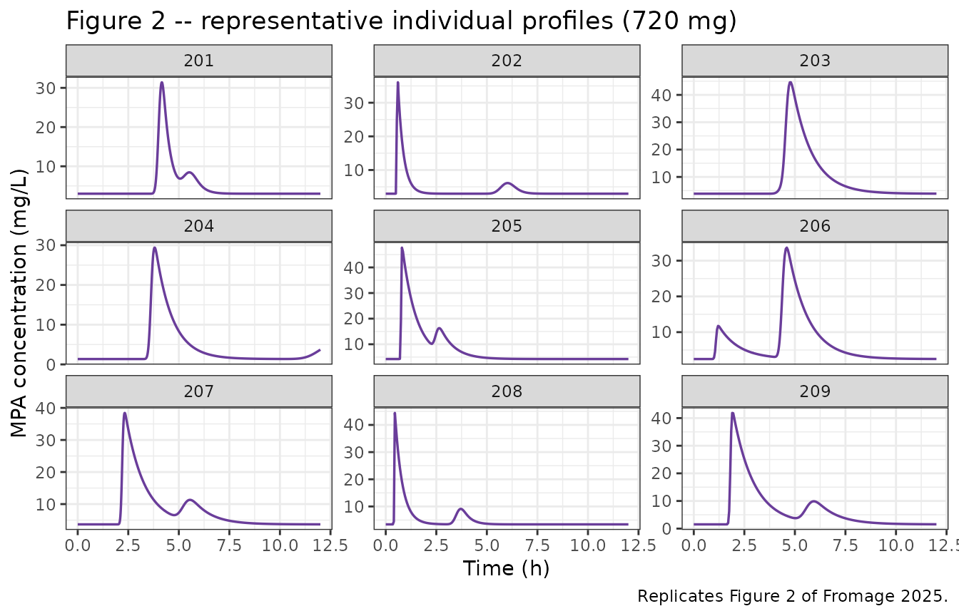
# Replicates Figure 4 of Fromage 2025: prediction-corrected VPC. Shown here as
# the simulated 10th / 50th / 90th percentiles by dose arm (the source overlays
# observed data that are not publicly available).
sim |>
  dplyr::group_by(arm, time) |>
  dplyr::summarise(Q10 = quantile(Cc, 0.10), Q50 = quantile(Cc, 0.50),
                   Q90 = quantile(Cc, 0.90), .groups = "drop") |>
  ggplot(aes(time, Q50)) +
  geom_ribbon(aes(ymin = Q10, ymax = Q90), alpha = 0.25, fill = "#1f78b4") +
  geom_line(colour = "#1f78b4", linewidth = 0.7) +
  facet_wrap(~arm) +
  labs(x = "Time (h)", y = "MPA concentration (mg/L)",
       title = "Figure 4 -- simulated prediction interval by dose arm",
       caption = paste("Replicates the prediction-interval component of",
                       "Figure 4 of Fromage 2025 (10th to 90th percentile).")) +
  theme_bw()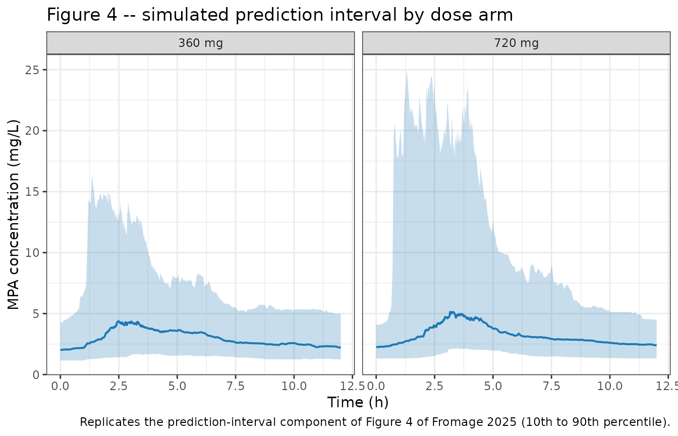
The simulated profiles show the shoulder-then-peak shape the
double-gamma model was chosen for, and the wide prediction interval
reflects the large IIV on the absorption rate constants (SD 0.92 on
log(b1)).
PKNCA validation
NCA is computed over the 0 to 12 h steady-state dosing interval.
cmin is used rather than ctrough because
ctrough is all-NA on a steady-state interval
of this shape.
sim_nca <- sim |>
  dplyr::filter(!is.na(Cc)) |>
  dplyr::select(id, time, Cc, arm)

# Guarantee a time = 0 row per (id, arm) so AUC0-12 is anchored. For this model
# the time-zero concentration is the trough C0, not zero, so keep the simulated
# value where one exists rather than overwriting it.
sim_nca <- dplyr::bind_rows(
  sim_nca,
  sim_nca |> dplyr::distinct(id, arm) |> dplyr::mutate(time = 0, Cc = p$C0)
) |>
  dplyr::distinct(id, arm, time, .keep_all = TRUE) |>
  dplyr::arrange(id, arm, time)

conc_obj <- PKNCA::PKNCAconc(sim_nca, Cc ~ time | arm + id)

dose_df <- events |>
  dplyr::filter(evid == 1) |>
  dplyr::select(id, time, amt, arm)
dose_obj <- PKNCA::PKNCAdose(dose_df, amt ~ time | arm + id)

intervals <- data.frame(start = 0, end = 12,
                        cmax = TRUE, tmax = TRUE, cmin = TRUE, auclast = TRUE)

nca_res <- PKNCA::pk.nca(PKNCA::PKNCAdata(conc_obj, dose_obj,
                                          intervals = intervals))

nca_wide <- as.data.frame(nca_res) |>
  dplyr::select(arm, id, PPTESTCD, PPORRES) |>
  tidyr::pivot_wider(names_from = PPTESTCD, values_from = PPORRES)

stopifnot(nrow(nca_wide) == 2L * n_per_arm, !anyNA(nca_wide$auclast))

nca_wide |>
  dplyr::group_by(arm) |>
  dplyr::summarise(
    `Cmax (mg/L)`       = mean(cmax),
    `Tmax (h)`          = median(tmax),
    `Cmin (mg/L)`       = mean(cmin),
    `AUC0-12 (mg*h/L)`  = mean(auclast),
    .groups = "drop"
  ) |>
  dplyr::rename("Dose arm" = arm) |>
  knitr::kable(digits = 2,
caption = "Simulated steady-state NCA by dose arm (n = 200 per arm).")| Dose arm | Cmax (mg/L) | Tmax (h) | Cmin (mg/L) | AUC0-12 (mg*h/L) |
|---|---|---|---|---|
| 360 mg | 18.83 | 2.92 | 2.47 | 46.88 |
| 720 mg | 34.28 | 3.09 | 2.51 | 61.48 |
Comparison against published values
Fromage 2025 does not tabulate Cmax, Tmax or AUC, so the comparison
targets the two derived quantities the Abstract does report:
CL/F = 4.99 +/- 2.22 L/h and
Vd/F = 12.60 +/- 0.08 L (mean +/- SD). The paper defines
CL/F = Dose / AUC (Section 2.2.1), which is computed below
from the PKNCA auclast over the dosing interval.
clf <- nca_wide |>
  dplyr::mutate(dose = dplyr::if_else(arm == "360 mg", 360, 720),
                clf = dose / auclast)

comparison <- clf |>
  dplyr::group_by(arm) |>
  dplyr::summarise(Simulated = mean(clf), `Simulated SD` = sd(clf),
                   .groups = "drop") |>
  dplyr::mutate(Quantity = paste0("CL/F, ", arm, " (L/h)"),
                Published = 4.99, `Published SD` = 2.22) |>
  dplyr::select(Quantity, Simulated, `Simulated SD`, Published, `Published SD`) |>
  dplyr::bind_rows(tibble::tibble(
    Quantity = "Vd/F (L)", Simulated = 100 / p$FAIV, `Simulated SD` = NA_real_,
    Published = 12.60, `Published SD` = 0.08))

comparison |>
  dplyr::mutate(`Ratio sim/pub` = Simulated / Published) |>
  knitr::kable(digits = 2,
               caption = paste("Simulated vs published derived parameters.",
"CL/F is Dose/AUC0-12 per the paper's definition."))| Quantity | Simulated | Simulated SD | Published | Published SD | Ratio sim/pub |
|---|---|---|---|---|---|
| CL/F, 360 mg (L/h) | 8.71 | 3.13 | 4.99 | 2.22 | 1.75 |
| CL/F, 720 mg (L/h) | 12.99 | 4.34 | 4.99 | 2.22 | 2.60 |
| Vd/F (L) | 12.71 | NA | 12.60 | 0.08 | 1.01 |
Vd/F matches to 0.9%. CL/F needs
interpretation, and the reason is structural rather than a defect:
because C0 is a dose-independent additive
offset, it contributes a fixed 12 * C0 = 26.5 mg*h/L to
every AUC0-12 regardless of dose, so Dose/AUC is
necessarily dose-dependent under this model. Evaluating the
typical-value profile across the source’s full dose range makes the
pattern explicit:
dose_scan <- lapply(c(180, 360, 540, 720, 1080, 1440), function(d) {
  s <- rxode2::rxSolve(mod_typ, make_events(d, ref_cov, times_fine))
  auc <- sum(diff(s$time) * (head(s$Cc, -1) + tail(s$Cc, -1)) / 2)
  tibble::tibble(`Dose (mg)` = d, `AUC0-12 (mg*h/L)` = auc,
                 `CL/F = Dose/AUC (L/h)` = d / auc)
}) |> dplyr::bind_rows()
#> ℹ omega/sigma items treated as zero: 'etalmtt1', 'etalmtt2', 'etalvc', 'etalkel', 'etalrbase'
#> ℹ omega/sigma items treated as zero: 'etalmtt1', 'etalmtt2', 'etalvc', 'etalkel', 'etalrbase'
#> ℹ omega/sigma items treated as zero: 'etalmtt1', 'etalmtt2', 'etalvc', 'etalkel', 'etalrbase'
#> ℹ omega/sigma items treated as zero: 'etalmtt1', 'etalmtt2', 'etalvc', 'etalkel', 'etalrbase'
#> ℹ omega/sigma items treated as zero: 'etalmtt1', 'etalmtt2', 'etalvc', 'etalkel', 'etalrbase'
#> ℹ omega/sigma items treated as zero: 'etalmtt1', 'etalmtt2', 'etalvc', 'etalkel', 'etalrbase'

knitr::kable(dose_scan, digits = 2,
             caption = paste("Typical-value CL/F across the source's dose range",
"(180 to 1440 mg per intake)."))| Dose (mg) | AUC0-12 (mg*h/L) | CL/F = Dose/AUC (L/h) |
|---|---|---|
| 180 | 34.35 | 5.24 |
| 360 | 42.17 | 8.54 |
| 540 | 50.00 | 10.80 |
| 720 | 57.83 | 12.45 |
| 1080 | 73.48 | 14.70 |
| 1440 | 89.13 | 16.16 |
The typical-value CL/F runs from 5.2 L/h at the lowest
studied intake (180 mg) to 16.2 L/h at the highest (1440 mg). The
published mean of 4.99 L/h therefore sits at the low-dose
end of the model’s own range. Two factors plausibly account for
this without any parameter being wrong: the published figure is an
arithmetic mean of individual Dose/AUC values over
a cohort with a right-skewed AUC distribution (large IIV on
C0, lambda and b1), and low-dose
occasions – where Dose/AUC is smallest – are heavily
represented (Table 1 median intake 360 mg, minimum 180 mg). No parameter
was adjusted to close the gap; the discrepancy is reported as found.
Assumptions and deviations
-
C0is a constant offset, not a decaying initial condition. The closed form addsC0outside theexp(-lambda*t)term, and the paper defines it as “the estimated trough concentration at steady state”. Reading it as a decaying initial condition is falsified twice over: withlambda = 1.81 1/h(t1/2 = 0.38 h) a decayingC0would be indistinguishable from zero by 12 h, contradicting the ~2 mg/L troughs in Figure 2; and it would implyCL/Faround 21 to 23 L/h at every plausible dose, against the Abstract’s 4.99 L/h. -
FAIVis normalised per 100 mg. It is reported in mg/L and the paper printsV/F = 100/FAIV, so the closed form’sFAIV * Damplitude isD/vcwithvc = 100/FAIV = 12.71 L. This is what reproduces the Abstract’sVd/F = 12.60 L. -
Gamma parameters stored as
(ntr, mtt). The bijectiona = ntr + 1,b = a/mttkeeps the canonical transit parameterisation used byDebord_2001_cyclosporin.R(the same group’s gamma absorption model) while remaining exactly the paper’s(a, b). Becauseacarries no IIV, the paper’s IIV onlog(b)and its covariate effect onlog(b2)transfer tolog(mtt)with a sign flip and unchanged variance; the sign inversion is recorded in theini()comments and verified in Gate 3. -
Single dosing interval only.
tad()/podo()refer to the most recent dose, so each dose restarts the absorption input and there is no superposition. The model must not be used to build up accumulation across doses;C0already represents the steady-state carry-over. -
Inter-occasion variability is not encoded. Table 2
reports IOV on
b1(SD 1.08, RSE 28.5%), estimated from sequential visits. Library model files omit IOV by nlmixr2lib convention, since no occasion column is assumed; a user who needs it can add an IOV term onlmtt1with variance 1.08^2. The authors themselves caution that highly variable visit intervals (mean 201 days, range 2 to 813) may have biased this estimate. -
The autoimmune-disease effect is retained despite being
non-significant. Section 3.2.2 reports
beta_b2_autoimmunewith 188% RSE and states it “can be disregarded”, but Section 4 confirms the authors “retained it in the model used for pcVPC simulations”. It is retained here for fidelity to the model the authors simulated from. Users wanting the reduced model can sete_dis_autoimmune_mtt2to 0. -
Covariates screened but not retained (sex, age,
time since transplantation, immunosuppressive co-medication, analytical
method) are recorded in the model file’s
covariatesDataExcludedlist rather thancovariateData, preserving the provenance of the covariate screen without declaring covariates thatmodel()never references. - Body weight, albumin and creatinine clearance are absent. These are the covariates most often reported to affect MPA clearance, but the ISBA extraction did not contain them (Section 4), so the model has no weight scaling. This limits extrapolation to the paediatric tail of the cohort (youngest 6 years) even though such patients contributed data.
- Virtual cohort composition. Both arms use the reference renal / hepatic indication and differ only in dose, so the dose comparison is not confounded by the absorption covariate. Sex, age and race are not model covariates and are therefore not simulated.
Errata
-
MAT2 for the reference group. The Discussion states
that
b2values of 95.69, 172.62 and 80.73 1/h give MAT2 of “4.09 h, 2.29 h and 4.90 h” respectively. Witha2 = 395.34from Table 2,a2/b2gives 4.13 h, 2.29 h and 4.90 h. The two covariate-group values reproduce exactly from the samea2, and no singlea2reproduces all three printed values, so 4.09 h is a rounding or transcription slip in the paper rather than a different parameter set. The packaged model implies 4.13 h; Gate 2 reports both numbers. -
Numerical note on the closed form versus an ODE.
The published closed form is used, not an equivalent ODE, partly because
it is what was fitted and partly for robustness:
a1 = 1280.97makes the first gamma component a near-delta pulse of width ~0.086 h, and integrating the corresponding ODE drives the central amount through denormal magnitudes (~1e-181) before the pulse arrives. With rxode2 5.1.7 that collapses lsoda’s step size, and on output grids finer than about 0.02 h the ODE formulation returns no absorption at all –Ccflat at the trough offset, with no error or warning under the defaultliblsoda– unlessatolis loosened to 1e-4 or larger. The closed form has no such failure mode and agrees with an independentpgamma()evaluation to 7e-15 mg/L at every grid density tested. The assertion in the Simulation chunk above guards against a silent recurrence.