Model and source
- Citation: Sun K, Jomphe C, Gosselin NH, Pheng L, Durairaj C, Hang Y, Bhattacharya I. Population Pharmacokinetics and Exposure-Response Relationships of Maribavir in Transplant Recipients With First Episode or Refractory Cytomegalovirus. CPT Pharmacometrics Syst Pharmacol. 2025;14(8):1346-1356. doi:10.1002/psp4.70054. Final NONMEM control stream in Supporting Information (file s001).
- Description: Updated two-compartment population PK model for oral maribavir in healthy volunteers, phase I special populations, and hematopoietic cell transplant (HCT) or solid organ transplant (SOT) recipients with cytomegalovirus (CMV) infection (Sun 2025, n = 930, 7431 concentration records pooled across phase 1, 2 and 3 studies including AURORA and SOLSTICE). First-order absorption with an absorption lag time, first-order elimination, estimated (not fixed) allometric body-weight exponents on CL/F, Vc/F, Q/F and Vp/F, strong CYP3A4 inhibitor and inducer effects and a CMV disease-state effect on CL/F, a dose effect on Ka, and proton-pump-inhibitor effects on both Ka and relative bioavailability. Supersedes the earlier pooled analysis extracted as Sun_2023_maribavir: the weight exponents are estimated here, and the PPI effects on F and Ka are new. The sixteen exposure-response logistic regressions reported alongside this PK model are extracted as the companion Sun_2025_maribavir_* family, which consumes this model’s individual exposures as their AUC_MBV_SS and AUC_MBV_DAY covariate columns.
- Article: https://doi.org/10.1002/psp4.70054
- Supporting Information (file
s001, which contains the final NONMEM control stream plus Tables S1-S4): https://doi.org/10.1002/psp4.70054
Maribavir is an orally bioavailable benzimidazole riboside with a selective multimodal mechanism of action against human cytomegalovirus (CMV). Sun 2025 is an update of a previously published pooled population PK analysis: it adds the randomized, double-blind phase 3 AURORA study in hematopoietic cell transplant (HCT) recipients with first asymptomatic CMV infection, and a phase 1 study in Japanese-descended and non-Hispanic Caucasian individuals. Relative to the earlier analysis the allometric body-weight exponents are now estimated rather than fixed, and proton-pump-inhibitor (PPI) effects on both relative bioavailability and the absorption rate constant are new.
A companion model from the same programme,
modellib("Sun_2023_maribavir"), encodes the earlier pooled
analysis that supported the adolescent dosing recommendation. The two
are not interchangeable: that one fixes the weight
exponents at 0.75 / 1 and carries no PPI effect.
This vignette covers seventeen models from one
paper. The population PK model is validated first; the sixteen
exposure-response logistic regressions that Sun 2025 fitted to the phase
3 AURORA arm are packaged as the Sun_2025_maribavir_*
family and validated in the Exposure-response models section
below, which also closes the loop by feeding PK-simulated exposures into
the efficacy model.
mod <- rxode2::rxode(readModelDb("Sun_2025_maribavir"))
mod
#>  ── rxode2-based free-form 3-cmt ODE model ──────────────────────────────────────
#>  ── Initalization: ──
#> Fixed Effects ($theta):
#>             lcl             lvc              lq             lvp             lka
#>      1.37118072      2.87919846      0.21511138      1.96009478     -0.36096987
#>           ltlag         lfdepot         e_wt_cl         e_wt_vc e_cyp3a4_inh_cl
#>     -1.55116900      0.00000000      0.30100000      0.53600000     -0.34389975
#> e_cyp3a4_ind_cl    e_dis_cmv_cl       e_dose_ka        e_ppi_ka         e_ppi_f
#>      0.81977983     -0.38860799     -1.02000000     -0.78307189     -0.09982034
#>           addSd    propSdPhase1   propSdPhase23
#>      0.01058301      0.26551836      0.39749214
#>
#> Omega ($omega):
#>              etalcl     etalvc     etalq    etalvp     etalka   etaltlag
#> etalcl   0.21915560 0.07966004 0.0000000 0.0000000  0.0000000  0.0000000
#> etalvc   0.07966004 0.06400900 0.0000000 0.0000000  0.0000000  0.0000000
#> etalq    0.00000000 0.00000000 1.1322082 0.7773213  0.0000000  0.0000000
#> etalvp   0.00000000 0.00000000 0.7773213 0.7929925  0.0000000  0.0000000
#> etalka   0.00000000 0.00000000 0.0000000 0.0000000  0.4176571 -0.2048004
#> etaltlag 0.00000000 0.00000000 0.0000000 0.0000000 -0.2048004  0.2136135
#>
#> States ($state or $stateDf):
#>   Compartment Number Compartment Name
#> 1                  1            depot
#> 2                  2          central
#> 3                  3      peripheral1
#>  ── μ-referencing ($muRefTable): ──
#>   theta      eta level
#> 1   lcl   etalcl    id
#> 2   lvc   etalvc    id
#> 3    lq    etalq    id
#> 4   lvp   etalvp    id
#> 5   lka   etalka    id
#> 6 ltlag etaltlag    id
#>                                                                                            covariates
#> 1 DIS_CMV*e_dis_cmv_cl + CONMED_CYP3A4_IND*e_cyp3a4_ind_cl + CONMED_CYP3A4_INH_STRONG*e_cyp3a4_inh_cl
#> 2
#> 3
#> 4
#> 5                                                                                 CONMED_PPI*e_ppi_ka
#> 6
#>
#>  ── Model (Normalized Syntax): ──
#> function() {
#>     compartmentData <- list(depot = list(analyte = "maribavir",
#>         units = "mg", specimen = "administration site", verified = TRUE),
#>         central = list(analyte = "maribavir", units = "mg", specimen = "plasma",
#>             verified = TRUE), peripheral1 = list(analyte = "maribavir",
#>             units = "mg", specimen = "plasma", verified = TRUE))
#>     covariateData <- list(WT = list(description = "Baseline body weight",
#>         units = "kg", type = "continuous", reference_category = NULL,
#>         notes = "Allometric power scaling with a 70 kg reference on all four disposition parameters. Unlike the earlier Sun 2023 analysis, which fixed the exponents at 0.75 and 1, this model ESTIMATED them, because the dataset now contains one individual under 18 years of age and the model was to support dose selection for an ongoing paediatric phase 3 study. The estimated exponents are smaller than the usual theoretical values: 0.301 for the clearance terms and 0.536 for the volume terms. The supplement control stream shows that Q/F reuses the CL/F weight coefficient (MU_3 = THETA(3) + CLWT) and Vp/F reuses the Vc/F weight coefficient (MU_4 = THETA(4) + VCWT) -- THETA(9) and THETA(10) are present but commented 'Not used'. This is why Table 2 reports identical estimates, %RSE and 95% CI for the CL/F and Q/F weight rows and again for the Vc/F and Vp/F rows: they are ONE parameter each, not two that happen to agree. The model file therefore carries two weight exponents, not four. Overall median 73.0 kg (range 36.1-141), Table 1.",
#>         source_name = "WTBL"), DOSE = list(description = "Administered maribavir dose per administration",
#>         units = "mg", type = "continuous", reference_category = NULL,
#>         notes = "Use case (a) of the DOSE canonical: the per-administration assigned dose level entering a power-form covariate effect on the first-order absorption rate, Ka = 0.697 * (DOSE/800)^-1.02, normalised at 800 mg. The exponent is negative, so Ka decreases as the dose increases. The control stream comment notes 'dose time changing for a few subjects', i.e. the column is per-record rather than strictly per-subject. Doses in the pooled dataset span single doses of 50-1600 mg (phase 1) and twice-daily regimens up to 1200 mg; the recommended clinical dose is 400 mg twice daily.",
#>         source_name = "DOSE"), DIS_CMV = list(description = "Transplant recipient with cytomegalovirus infection/disease indicator",
#>         units = "(binary)", type = "binary", reference_category = "0 (healthy volunteer / non-CMV phase 1 participant)",
#>         notes = "1 = HCT or SOT recipient with CMV infection (the phase 2/3 and AURORA populations, n = 724); 0 = healthy volunteer or phase 1 participant without CMV, including the renal- and hepatic-impairment cohorts (n = 206). Derived in the control stream as HSCMV = 1 when the health status column HS equals 2, with the comment ';HV reference' marking the healthy volunteer as the reference level. Enters as a log-scale additive shift on CL/F: CL/F is 0.678x lower in transplant recipients with CMV, i.e. clearance is 32% lower, which the authors attribute to reduced liver and/or kidney function and concurrent medications. Note that transplant TYPE (HCT vs SOT, and organ within SOT) was tested and was NOT a significant predictor, so this covariate carries the whole patient-vs-healthy contrast.",
#>         source_name = "HSCMV"), CONMED_CYP3A4_INH_STRONG = list(description = "Concomitant strong CYP3A4 inhibitor coadministration indicator",
#>         units = "(binary)", type = "binary", reference_category = "0 (no strong CYP3A4 inhibitor coadministration)",
#>         notes = "Time-varying per record (Table 1 footnote b: the same individual may appear as both No and Yes). Multiplicative power-form effect on CL/F: 0.709^CONMED_CYP3A4_INH_STRONG, a 29% reduction in CL/F, which the authors note is consistent with the 35% reduction seen in the dedicated ketoconazole DDI study. 129 of 930 individuals (13%) had strong inhibitor exposure. The STRONG-specific canonical is used rather than the class-level CONMED_CYP3A4_INH because this analysis screened strong and moderate inhibitors separately (Table 1 lists both) and retained only the strong effect; the moderate-inhibitor coefficient THETA(20) is '(1) FIX' in the control stream, i.e. no effect. See covariatesDataExcluded$CONMED_CYP3A4_INH_MOD.",
#>         source_name = "CYP3AINH"), CONMED_CYP3A4_IND = list(description = "Concomitant strong CYP3A4 inducer coadministration indicator",
#>         units = "(binary)", type = "binary", reference_category = "0 (no CYP3A4 inducer coadministration)",
#>         notes = "Time-varying per record. Multiplicative power-form effect on CL/F: 2.27^CONMED_CYP3A4_IND, a 2.27-fold increase in CL/F, which the authors note is consistent with the 2.5-fold increase seen in the dedicated rifampin DDI study. Table 1 labels the covariate 'Strong CY3A4 inducers' (18 of 930 individuals, 2%); the paper states explicitly that there were insufficient patients receiving moderate and weak inducers to evaluate their effect, so no strength-stratified inducer canonical is used and the class-level column carries the strong-inducer effect.",
#>         source_name = "CYP3AIND"), CONMED_PPI = list(description = "Concomitant proton-pump inhibitor use indicator",
#>         units = "(binary)", type = "binary", reference_category = "0 (no proton-pump inhibitor coadministration)",
#>         notes = "Time-varying per record (Table 1 footnote b). New in this analysis relative to the earlier Sun 2023 model. Carries TWO effects, both multiplicative on the natural scale and both entered in the control stream as EXP(THETA) gates: relative bioavailability F = 0.905^PPI (F1 = PPIF) and absorption rate Ka = ... * 0.457^PPI (KA = ... * PPIKA). Because a lower F lowers exposure while a lower Ka flattens and delays the profile, the net effect is -9.5% on AUCss and -22.5% on Cmax,ss with essentially no change in Cmin,ss (Figure 2b) -- which the authors judge to be of little clinical significance given maribavir's flat exposure-response. 529 of 973 records-level classifications (54%) were PPI-exposed, the most prevalent co-medication in the analysis.",
#>         source_name = "PPI"), STUDY_MARIBAVIR_PHASE1 = list(description = "Phase 1 study cohort indicator",
#>         units = "(binary)", type = "binary", reference_category = "0 (phase 2/3 study: SHP620-202, -203, -302, -303 and AURORA)",
#>         notes = "1 = the concentration record originates from a phase 1 study (n = 206 individuals, 4231 records); 0 = a phase 2/3 study. Used ONLY to switch the proportional residual-error magnitude, exactly as in the control stream $ERROR block, which selects EPS(3) instead of EPS(1) when STUDY is 202, 203, 302 or 303. The authors attribute the difference to the different LC-MS assays, with different lower limits of quantification, used in the phase 1 versus the phase 2/3 studies. This column has no structural effect: it does not enter any PK parameter.",
#>         source_name = "STUDY"))
#>     covariatesDataExcluded <- list(CONMED_CYP3A4_INH_MOD = list(description = "Concomitant moderate CYP3A4 inhibitor coadministration indicator",
#>         units = "(binary)", type = "binary", reference_category = "0 (no moderate CYP3A4 inhibitor coadministration)",
#>         notes = "Screened as a multiplicative effect on CL/F via THETA(20), labelled '[CL~CYPMOD]', but the coefficient is '(1) FIX' -- a multiplier of exactly 1, i.e. no effect. The control-stream header line ';; 1. Based on: noCYPINHmCL' records that this run is the one built WITHOUT the moderate-CYP-inhibitor effect on CL. 103 of 930 individuals (11%) had moderate-inhibitor exposure (Table 1). Not reported in Table 2.",
#>         source_name = "CYP3AIHM"), SEXF = list(description = "Female sex indicator",
#>         units = "(binary)", type = "binary", reference_category = "0 (male)",
#>         notes = "Screened as an effect on both CL/F (THETA(14)) and Vc/F (THETA(15)) in the final control stream, but both coefficients are '(0) FIX'. The Discussion states there was no evidence that sex affected maribavir PK. Note that Figure 2a nonetheless shows ~24% higher steady-state exposure in females than males; that is a body-weight-mediated difference propagated through the allometric terms, not a separate sex effect. 930 individuals were 41% female (Table 1).",
#>         source_name = "SEXN"), HEPIMP_MOD = list(description = "Moderate hepatic impairment (Child-Pugh class B) indicator",
#>         units = "(binary)", type = "binary", reference_category = "0 (no moderate hepatic impairment)",
#>         notes = "Screened as an effect on Vc/F (THETA(13), labelled '[Vc~Child-Pugh Class B]') and derived in the control stream as HEPN2 = 1 when HEPN equals 2, but the coefficient is '(0) FIX'. 18 of 930 individuals were Child-Pugh class B (Table S1). The Discussion lists hepatic impairment among the covariates with no evidence of an effect on maribavir PK.",
#>         source_name = "HEPN2"))
#>     description <- "Updated two-compartment population PK model for oral maribavir in healthy volunteers, phase I special populations, and hematopoietic cell transplant (HCT) or solid organ transplant (SOT) recipients with cytomegalovirus (CMV) infection (Sun 2025, n = 930, 7431 concentration records pooled across phase 1, 2 and 3 studies including AURORA and SOLSTICE). First-order absorption with an absorption lag time, first-order elimination, estimated (not fixed) allometric body-weight exponents on CL/F, Vc/F, Q/F and Vp/F, strong CYP3A4 inhibitor and inducer effects and a CMV disease-state effect on CL/F, a dose effect on Ka, and proton-pump-inhibitor effects on both Ka and relative bioavailability. Supersedes the earlier pooled analysis extracted as Sun_2023_maribavir: the weight exponents are estimated here, and the PPI effects on F and Ka are new. The sixteen exposure-response logistic regressions reported alongside this PK model are extracted as the companion Sun_2025_maribavir_* family, which consumes this model's individual exposures as their AUC_MBV_SS and AUC_MBV_DAY covariate columns."
#>     paper_specific_residual_sds <- c("propSdPhase1", "propSdPhase23")
#>     population <- list(species = "human", n_subjects = 930L,
#>         n_studies = "Not stated as a single count. The pooled dataset spans phase 1 (n = 206), phase 2/3 (n = 724, which includes SOLSTICE), and AURORA (n = 238, a subset of the phase 2/3 group), plus a phase 1 study in Japanese-descended and non-Hispanic Caucasian individuals (NCT05319353) newly added in this update.",
#>         n_observations = 7431L, age_range = "12 to <18 years: 1 (<1%); 18 to <65 years: 761 (82%); 65 to <80 years: 168 (18%) (Table 1). The single individual under 18 is the reason the allometric exponents were estimated rather than fixed.",
#>         weight_range = "36.1-141 kg; median 73.0 kg, mean 74.2 kg (SD 17.4) (Table 1). AURORA weights not reported.",
#>         sex_female_pct = 41, race_ethnicity = c(Caucasian = 77,
#>             Black = 13, Asian = 7, Other = 3), disease_state = "Pooled analysis of healthy volunteers (157), phase 1 participants with hepatic impairment (10), renal impairment (19) or stable renal transplant (20), and HCT or SOT recipients with CMV infection (724). CMV category: no infection 206, asymptomatic infection 644, symptomatic infection 44, CMV organ disease 36. Transplant type: none 186, SOT 304, HCT 440.",
#>         dose_range = "Single doses of 50-1600 mg and multiple doses up to 2400 mg/day across the pooled phase 1-3 dataset; the recommended and most-represented regimen is 400 mg twice daily.",
#>         regions = "North America, Europe and Asia Pacific (region proportions reported only for the 238-patient AURORA exposure-response subset: North America 24.8%, Europe 58.0%, Asia Pacific 17.2%, Table S2).",
#>         co_medication = "Proton-pump inhibitors 54%, strong CYP3A4 inhibitors 13%, moderate CYP3A4 inhibitors 11%, histamine H2 blockers 10%, antacids 8%, weak CYP3A4 inhibitors 6%, strong CYP3A4 inducers 2% (Table 1 and Table S1).",
#>         notes = "Below-limit-of-quantification data were handled by method M1 (all 297 BLQ records, 3.5% of post-dose values, excluded). Parameters were estimated in NONMEM 7.5.1 with IMPMAP; standard errors and 95% non-parametric confidence intervals came from bootstrap stratified by study. Structure was read from the final control stream in Supporting Information file s001; every parameter VALUE comes from the published Table 2, because the control stream's $THETA / $OMEGA / $SIGMA blocks are the run's INITIAL estimates (they are close to but not equal to the final values -- e.g. THETA(16) [KA~dose] is -1.17 initially against a final -1.02, and -1.17 is in fact the lower bound of the published 95% CI).")
#>     reference <- "Sun K, Jomphe C, Gosselin NH, Pheng L, Durairaj C, Hang Y, Bhattacharya I. Population Pharmacokinetics and Exposure-Response Relationships of Maribavir in Transplant Recipients With First Episode or Refractory Cytomegalovirus. CPT Pharmacometrics Syst Pharmacol. 2025;14(8):1346-1356. doi:10.1002/psp4.70054. Final NONMEM control stream in Supporting Information (file s001)."
#>     units <- list(time = "h", dosing = "mg", concentration = "ug/mL")
#>     vignette <- "Sun_2025_maribavir"
#>     ini({
#>         lcl <- 1.37118072330984
#>         label("Apparent clearance in the reference subject (L/h)")
#>         lvc <- 2.87919845729804
#>         label("Apparent central volume of distribution in the reference subject (L)")
#>         lq <- 0.215111379616945
#>         label("Apparent intercompartmental clearance in the reference subject (L/h)")
#>         lvp <- 1.96009478404727
#>         label("Apparent peripheral volume of distribution in the reference subject (L)")
#>         lka <- -0.360969868221613
#>         label("First-order absorption rate at the 800 mg reference dose (1/h)")
#>         ltlag <- -1.55116900431012
#>         label("Absorption lag time (h)")
#>         lfdepot <- fix(0)
#>         label("Relative bioavailability in the reference subject (fraction)")
#>         e_wt_cl <- 0.301
#>         label("Allometric (WT/70) exponent shared by CL/F and Q/F (unitless)")
#>         e_wt_vc <- 0.536
#>         label("Allometric (WT/70) exponent shared by Vc/F and Vp/F (unitless)")
#>         e_cyp3a4_inh_cl <- -0.34389975245001
#>         label("Log-effect of concomitant strong CYP3A4 inhibitor on CL/F (unitless)")
#>         e_cyp3a4_ind_cl <- 0.819779831493311
#>         label("Log-effect of concomitant CYP3A4 inducer on CL/F (unitless)")
#>         e_dis_cmv_cl <- -0.388607991041741
#>         label("Log-effect of transplant-recipient-with-CMV status on CL/F (unitless)")
#>         e_dose_ka <- -1.02
#>         label("Power exponent of maribavir dose on Ka, normalised at 800 mg (unitless)")
#>         e_ppi_ka <- -0.783071888087932
#>         label("Log-effect of concomitant proton-pump inhibitor on Ka (unitless)")
#>         e_ppi_f <- -0.0998203352822109
#>         label("Log-effect of concomitant proton-pump inhibitor on F (unitless)")
#>         addSd <- c(0, 0.0105830052442584)
#>         label("Additive residual error, all studies (ug/mL)")
#>         propSdPhase1 <- 0.265518360947035
#>         label("Proportional residual error, phase 1 studies (fraction)")
#>         propSdPhase23 <- 0.397492138287036
#>         label("Proportional residual error, phase 2/3 studies (fraction)")
#>         etalcl ~ 0.2191556
#>         etalvc ~ c(0.07966004, 0.064009)
#>         etalq ~ 1.1322082
#>         etalvp ~ c(0.7773213, 0.7929925)
#>         etalka ~ 0.4176571
#>         etaltlag ~ c(-0.2048004, 0.2136135)
#>     })
#>     model({
#>         cl <- exp(lcl + e_cyp3a4_inh_cl * CONMED_CYP3A4_INH_STRONG +
#>             e_cyp3a4_ind_cl * CONMED_CYP3A4_IND + e_dis_cmv_cl *
#>             DIS_CMV + etalcl) * (WT/70)^e_wt_cl
#>         vc <- exp(lvc + etalvc) * (WT/70)^e_wt_vc
#>         q <- exp(lq + etalq) * (WT/70)^e_wt_cl
#>         vp <- exp(lvp + etalvp) * (WT/70)^e_wt_vc
#>         ka <- exp(lka + e_ppi_ka * CONMED_PPI + etalka) * (DOSE/800)^e_dose_ka
#>         tlag <- exp(ltlag + etaltlag)
#>         fdepot <- exp(lfdepot + e_ppi_f * CONMED_PPI)
#>         kel <- cl/vc
#>         k12 <- q/vc
#>         k21 <- q/vp
#>         d/dt(depot) <- -ka * depot
#>         d/dt(central) <- ka * depot - kel * central - k12 * central +
#>             k21 * peripheral1
#>         d/dt(peripheral1) <- k12 * central - k21 * peripheral1
#>         alag(depot) <- tlag
#>         f(depot) <- fdepot
#>         Cc <- central/vc
#>         propSd <- propSdPhase1 * STUDY_MARIBAVIR_PHASE1 + propSdPhase23 *
#>             (1 - STUDY_MARIBAVIR_PHASE1)
#>         Cc ~ prop(propSd) + add(addSd)
#>     })
#> }
Population
The parameter-estimation population is 930 individuals contributing 7431 maribavir plasma concentration records, pooled across phase 1, 2 and 3 studies (Sun 2025 Table 1 and Section 3.1):
- Phase 1 (n = 206, 4231 records) – 157 healthy volunteers, 19 with renal impairment, 20 stable renal transplant recipients and 10 with hepatic impairment. None have CMV infection.
- Phase 2/3 (n = 724, 3200 records) – HCT (440) and solid organ transplant (SOT, 284) recipients with CMV infection, including the SOLSTICE refractory population. CMV category: asymptomatic 644, symptomatic 44, organ disease 36.
- AURORA (n = 238) – a subset of the phase 2/3 group; all HCT recipients with first asymptomatic CMV infection. This is the cohort newly added in this update and the cohort used for the exposure-response analyses.
Demographics: 82% aged 18 to <65 years and 18% aged 65 to <80, with a single individual under 18 – that one individual is the stated reason the allometric exponents were estimated rather than fixed, in support of an ongoing paediatric phase 3 study. Weight median 73.0 kg (range 36.1-141), mean 74.2 (SD 17.4). 41% female. Race: Caucasian 77%, Black 13%, Asian 7%, Other 3%.
Co-medication prevalence is high and matters for this model: PPIs 54%, strong CYP3A4 inhibitors 13%, moderate CYP3A4 inhibitors 11%, H2 blockers 10%, antacids 8%, strong CYP3A4 inducers 2%.
Below-limit-of-quantification records (297; 3.5% of post-dose values) were excluded under method M1. Estimation used NONMEM 7.5.1 with IMPMAP; confidence intervals came from non-parametric bootstrap stratified by study.
Source trace
Every ini() value comes from the published Table 2. The
model structure comes from the final NONMEM control
stream in Supporting Information file s001. The distinction
matters: the control stream’s $THETA / $OMEGA
/ $SIGMA blocks are that run’s initial estimates,
not its final ones – for example THETA(16) [KA~dose] is
-1.17 there against a published final -1.02,
and -1.17 is in fact the lower bound of the published 95%
CI. Values therefore come from the table, structure from the code.
| Model element | Source location | Value |
|---|---|---|
| CL/F reference | Table 2 CL/F (L/h)
|
3.94 (95% CI 3.69-4.20) |
| Vc/F reference | Table 2 Vc/F (L)
|
17.8 (16.9-18.9) |
| Q/F reference | Table 2 Q/F (L/h)
|
1.24 (0.962-1.60) |
| Vp/F reference | Table 2 Vp/F (L)
|
7.10 (6.04-8.35) |
| Ka at 800 mg | Table 2 Ka (1/h)
|
0.697 (0.594-0.819) |
| Absorption lag | Table 2 Lag (h)
|
0.212 (0.192-0.235) |
| F reference | Table 2 F
|
1 (no uncertainty reported; fixed()) |
| WT exponent, CL/F and Q/F | Table 2 Effect of WT on CL/F =
Effect of WT on Q/F; control stream
MU_3 = THETA(3) + CLWT
|
0.301 (0.159-0.443) |
| WT exponent, Vc/F and Vp/F | Table 2 Effect of WT on Vc/F =
Effect of WT on Vp/F; control stream
MU_4 = THETA(4) + VCWT
|
0.536 (0.378-0.694) |
| Strong CYP3A4 inhibitor on CL/F | Table 2 Effect of CYP3AINH on CL/F
|
x0.709 (0.681-0.737) |
| CYP3A4 inducer on CL/F | Table 2 Effect of CYP3AIND on CL/F
|
x2.27 (2.15-2.38) |
| CMV status on CL/F | Table 2 Effect of CMV on CL/F
|
x0.678 (0.626-0.733) |
| Dose on Ka | Table 2 Effect of dose on Ka
|
x(DOSE/800)^-1.02 (-1.17 to -0.875) |
| PPI on Ka | Table 2 Effect of PPI on Ka
|
x0.457 (0.367-0.568) |
| PPI on F | Table 2 Effect of PPI on F
|
x0.905 (0.849-0.964) |
| IIV diagonals (6) | Table 2 IIV (%) column |
49.5, 25.3, 145, 110, 72.0, 48.8% |
| IIV block structure | Control stream 3 OMEGA BLOCK(2) over
ETA(1..6)
|
CL~Vc, Q~Vp, Ka~lag |
| IIV off-diagonals |
Not published; correlations carried from the
control stream $OMEGA initial estimates |
r = 0.673, 0.820, -0.686 |
| Additive residual | Table 2 sigma^2 add
|
0.000112 -> SD 0.010583 |
| Proportional residual, phase 1 | Table 2 sigma^2 prop Phase 1
|
0.0705 -> SD 0.265518 |
| Proportional residual, phase 2/3 | Table 2 sigma^2 prop Phase 2 & 3
|
0.158 -> SD 0.397492 |
Structural model, $ERROR, F1 = PPIF,
ALAG1
|
Control stream (ADVAN4 TRANS4) |
– |
Two structural readings deserve emphasis, because Table 2 alone is ambiguous about both and only the control stream settles them.
Two weight exponents, not four. Table 2 lists four
weight rows, but the CL/F and Q/F rows carry identical
estimates, %RSE and 95% CI, as do the Vc/F and Vp/F rows. That is not a
coincidence of rounding: the control stream computes CLWT
and VCWT once and reuses them
(MU_3 = THETA(3) + CLWT,
MU_4 = THETA(4) + VCWT), while THETA(9) and
THETA(10) are present but commented Not used.
The model file therefore has two exponent parameters.
The IIV (%) back-transform. Table 2
reports IIV as a percentage without stating the convention. This file
uses the rule that the same analysis group documented explicitly for the
same drug in the companion Sun 2023 paper (its Table S2 footnote c):
CV = sqrt(omega^2) when omega^2 <= 0.15 and
CV = sqrt(exp(omega^2) - 1) otherwise. All six Table 2
entries are self-consistent under that rule, and only Vc/F falls in the
first branch, where the two branches differ by less than 2% in SD. The
two best-determined parameters corroborate it: back-transforming CL/F’s
49.5% gives omega^2 = 0.2192 against the control stream’s
initial 0.214, and the lag time’s 48.8% gives 0.2136 against an initial
0.203.
Virtual cohort
Two arms of 200 participants each, matching the two health-status strata that Sun 2025 Table 3 reports separately. Both are simulated at 400 mg twice daily without concomitant medication, which is exactly the condition Table 3 and Figure 2 state for their exposure summaries.
Weights are drawn from log-normal distributions matched to the per-stratum Table 1 summaries (phase 1 mean 78.1, SD 15.1; phase 2/3 mean 73.1, SD 17.8) and truncated to the reported overall range 36.1-141 kg.
set.seed(20250704)
rxode2::rxSetSeed(20250704)

n_arm <- 200L

draw_wt <- function(n, mean_kg, sd_kg) {
  sdlog <- sqrt(log1p((sd_kg / mean_kg)^2))
  meanlog <- log(mean_kg) - sdlog^2 / 2
  pmin(pmax(stats::rlnorm(n, meanlog, sdlog), 36.1), 141)
}

cohort <- dplyr::bind_rows(
  tibble::tibble(
    id        = seq_len(n_arm),
    treatment = "Healthy volunteers",
    WT        = draw_wt(n_arm, 78.1, 15.1),
    DIS_CMV   = 0,
    STUDY_MARIBAVIR_PHASE1 = 1
  ),
  tibble::tibble(
    id        = n_arm + seq_len(n_arm),
    treatment = "Transplant recipients with CMV",
    WT        = draw_wt(n_arm, 73.1, 17.8),
    DIS_CMV   = 1,
    STUDY_MARIBAVIR_PHASE1 = 0
  )
) |>
  dplyr::mutate(
    DOSE                     = 400,
    CONMED_PPI               = 0,
    CONMED_CYP3A4_INH_STRONG = 0,
    CONMED_CYP3A4_IND        = 0
  )

cohort |>
  dplyr::group_by(treatment) |>
  dplyr::summarise(
    n = dplyr::n(),
    `Weight mean (kg)`   = round(mean(WT), 1),
    `Weight median (kg)` = round(stats::median(WT), 1),
    `Weight SD (kg)`     = round(stats::sd(WT), 1),
    .groups = "drop"
  ) |>
knitr::kable(caption = "Simulated cohort weight distributions (Sun 2025 Table 1 targets: phase 1 mean 78.1 SD 15.1, median 75.6; phase 2/3 mean 73.1 SD 17.8, median 71.3).")| treatment | n | Weight mean (kg) | Weight median (kg) | Weight SD (kg) |
|---|---|---|---|---|
| Healthy volunteers | 200 | 78.6 | 77.1 | 13.9 |
| Transplant recipients with CMV | 200 | 71.4 | 70.4 | 16.3 |
Simulation
400 mg twice daily for 10 days (20 doses, ii = 12,
addl = 19), which is far beyond the 2 days to steady state
the paper reports for this regimen. The observation grid covers the
last dosing interval, 228-240 h, so the
non-compartmental interval is a true steady-state interval and its lower
bound carries a real pre-dose trough record rather than a synthetic
time-zero anchor.
events <- rxode2::et(amt = 400, ii = 12, addl = 19, cmt = "depot") |>
  rxode2::et(seq(228, 240, by = 0.1), cmt = "central") |>
  rxode2::et(id = cohort$id)

ev_df <- as.data.frame(events) |>
  dplyr::left_join(cohort, by = "id")

sim <- rxode2::rxSolve(mod, ev_df, returnType = "data.frame") |>
  dplyr::left_join(dplyr::select(cohort, id, treatment), by = "id")

str(dplyr::select(sim, id, time, Cc), max.level = 1)
#> 'data.frame':    48400 obs. of  3 variables:
#>  $ id  : int  1 1 1 1 1 1 1 1 1 1 ...
#>  $ time: num  228 228 228 228 228 ...
#>  $ Cc  : num  3.75 3.71 4.87 10 13.81 ...
Steady-state concentration-time profiles
sim |>
  dplyr::group_by(treatment, time) |>
  dplyr::summarise(
    med = stats::median(Cc),
    lo  = stats::quantile(Cc, 0.05),
    hi  = stats::quantile(Cc, 0.95),
    .groups = "drop"
  ) |>
  ggplot2::ggplot(ggplot2::aes(time - 228, med, colour = treatment, fill = treatment)) +
  ggplot2::geom_ribbon(ggplot2::aes(ymin = lo, ymax = hi), alpha = 0.2, colour = NA) +
  ggplot2::geom_line(linewidth = 1) +
  ggplot2::scale_y_log10() +
  ggplot2::labs(
    x = "Time after dose at steady state (h)",
    y = "Maribavir concentration (ug/mL)",
    colour = NULL, fill = NULL
  ) +
  ggplot2::theme(legend.position = "bottom")
Simulated steady-state maribavir profiles over the last 12 h dosing interval of 400 mg twice daily, by health status. Compare with the observed-versus-predicted spread in Sun 2025 Figure 1 (prediction-corrected VPC).
Structural checks (typical value, no random effects)
These are deterministic: zeroRe() removes both the
between-subject and the residual variability, so the numbers below
depend only on the ini() values and the
model() algebra. They are the sharpest available test of
the covariate encoding, and they are compared against numbers Sun 2025
reports directly.
mod_typ <- rxode2::zeroRe(mod)

typ_exposure <- function(ppi = 0, cmv = 1, wt = 70, dose = 400) {
  ev <- rxode2::et(amt = dose, ii = 12, addl = 19, cmt = "depot") |>
    rxode2::et(seq(228, 240, by = 0.01), cmt = "central")
  d <- as.data.frame(ev)
  d$WT <- wt
  d$DOSE <- dose
  d$DIS_CMV <- cmv
  d$CONMED_PPI <- ppi
  d$CONMED_CYP3A4_INH_STRONG <- 0
  d$CONMED_CYP3A4_IND <- 0
  d$STUDY_MARIBAVIR_PHASE1 <- 0
  s <- rxode2::rxSolve(mod_typ, d, returnType = "data.frame")
  s <- s[!is.na(s$Cc), ]
  c(
    auc  = sum(diff(s$time) * (utils::head(s$Cc, -1) + utils::tail(s$Cc, -1)) / 2),
    cmax = max(s$Cc),
    cmin = min(s$Cc)
  )
}

cmv_noppi <- typ_exposure(ppi = 0, cmv = 1)
#> ℹ omega/sigma items treated as zero: 'etalcl', 'etalvc', 'etalq', 'etalvp', 'etalka', 'etaltlag'
cmv_ppi   <- typ_exposure(ppi = 1, cmv = 1)
#> ℹ omega/sigma items treated as zero: 'etalcl', 'etalvc', 'etalq', 'etalvp', 'etalka', 'etaltlag'
healthy   <- typ_exposure(ppi = 0, cmv = 0)
#> ℹ omega/sigma items treated as zero: 'etalcl', 'etalvc', 'etalq', 'etalvp', 'etalka', 'etaltlag'
Steady-state mass balance
At steady state the amount cleared over one dosing interval must
equal the delivered dose, so AUCss x CL/F = F x Dose
exactly. This is the cheapest gate that would catch a mis-scaled volume,
a wrong concentration unit, or an rxode2
cl/vc pair silently replacing the explicit
ODEs with an analytical solution.
Covariate effect ratios against the published values
Sun 2025 quantifies three covariate contrasts numerically. Each is reproduced below from the model algebra alone. The PPI contrast is the strongest test in this vignette, because it is the net result of two separate effects pulling in different directions – bioavailability down 9.5% and absorption rate down 54.3% – and the paper reports its AUC, Cmax and Cmin consequences separately.
ratios <- tibble::tibble(
  Contrast = c(
    "PPI vs no PPI, AUCss", "PPI vs no PPI, Cmax,ss", "PPI vs no PPI, Cmin,ss",
    "CMV vs healthy, AUCss", "CMV vs healthy, Cmax,ss", "CMV vs healthy, Cmin,ss"
  ),
  Simulated = c(
    cmv_ppi["auc"] / cmv_noppi["auc"],
    cmv_ppi["cmax"] / cmv_noppi["cmax"],
    cmv_ppi["cmin"] / cmv_noppi["cmin"],
    cmv_noppi["auc"] / healthy["auc"],
    cmv_noppi["cmax"] / healthy["cmax"],
    cmv_noppi["cmin"] / healthy["cmin"]
  ),
  Published = c(0.905, 0.775, 1.03, 1.46, 1.20, 2.11),
  Source = c(
    "Figure 2b / Section 3.1.3 (-9.5%)", "Figure 2b / Section 3.1.3 (-22.5%)", "Figure 2b",
    "Section 3.1.3", "Section 3.1.3", "Section 3.1.3"
  )
) |>
  dplyr::mutate(
    Simulated = round(Simulated, 3),
    `% diff`  = round(100 * (Simulated - Published) / Published, 1)
  )

knitr::kable(ratios, caption = "Typical-value covariate contrasts against the values Sun 2025 reports.")| Contrast | Simulated | Published | Source | % diff |
|---|---|---|---|---|
| PPI vs no PPI, AUCss | 0.905 | 0.905 | Figure 2b / Section 3.1.3 (-9.5%) | 0.0 |
| PPI vs no PPI, Cmax,ss | 0.779 | 0.775 | Figure 2b / Section 3.1.3 (-22.5%) | 0.5 |
| PPI vs no PPI, Cmin,ss | 1.004 | 1.030 | Figure 2b | -2.5 |
| CMV vs healthy, AUCss | 1.475 | 1.460 | Section 3.1.3 | 1.0 |
| CMV vs healthy, Cmax,ss | 1.221 | 1.200 | Section 3.1.3 | 1.8 |
| CMV vs healthy, Cmin,ss | 2.134 | 2.110 | Section 3.1.3 | 1.1 |
# The PPI AUCss ratio is a pure function of the F effect and must reproduce
# 0.905 essentially exactly; the others involve absorption and distribution and
# are compared against population geometric-mean ratios, so they are given
# proportionally more headroom.
stopifnot(
  abs(ratios$`% diff`[1]) < 0.5,
  max(abs(ratios$`% diff`)) < 5
)
PKNCA validation
Non-compartmental analysis over the steady-state interval 228-240 h, grouped by treatment arm so each arm can be compared against its own Table 3 row.
conc_data <- sim |>
  dplyr::filter(!is.na(Cc)) |>
  dplyr::select(id, treatment, time, Cc)

dose_data <- cohort |>
  dplyr::transmute(id, treatment, time = 228, dose = 400)

o_conc <- PKNCA::PKNCAconc(conc_data, Cc ~ time | id / treatment)
# PKNCAdose does not accept slash (nested) grouping, only PKNCAconc does.
o_dose <- PKNCA::PKNCAdose(dose_data, dose ~ time | id + treatment)

intervals <- data.frame(
  start = 228, end = 240,
  auclast = TRUE, cmax = TRUE, cmin = TRUE, half.life = TRUE
)

o_nca <- PKNCA::pk.nca(PKNCA::PKNCAdata(o_conc, o_dose, intervals = intervals))

nca_res <- as.data.frame(o_nca) |>
  dplyr::filter(PPTESTCD %in% c("auclast", "cmax", "cmin", "half.life"))

stopifnot(nrow(nca_res) > 0L, !anyNA(nca_res$PPORRES))
nca_gm <- nca_res |>
  dplyr::group_by(treatment, PPTESTCD) |>
  dplyr::summarise(
    gm  = exp(mean(log(PPORRES))),
    cv  = 100 * sqrt(exp(stats::var(log(PPORRES))) - 1),
    .groups = "drop"
  )

nca_gm |>
  dplyr::mutate(
    Parameter = dplyr::recode(
      PPTESTCD,
      auclast     = "AUCss (ug*h/mL)",
      cmax        = "Cmax,ss (ug/mL)",
      cmin        = "Cmin,ss (ug/mL)",
      half.life   = "t1/2 (h)"
    ),
    `Geometric mean` = round(gm, 3),
    `CV%`            = round(cv, 1)
  ) |>
  dplyr::select(Arm = treatment, Parameter, `Geometric mean`, `CV%`) |>
knitr::kable(caption = "Simulated steady-state exposure at 400 mg twice daily without concomitant medication.")| Arm | Parameter | Geometric mean | CV% |
|---|---|---|---|
| Healthy volunteers | AUCss (ug*h/mL) | 95.272 | 48.9 |
| Healthy volunteers | Cmax,ss (ug/mL) | 15.760 | 36.8 |
| Healthy volunteers | Cmin,ss (ug/mL) | 2.627 | 106.3 |
| Healthy volunteers | t1/2 (h) | 5.184 | 43.8 |
| Transplant recipients with CMV | AUCss (ug*h/mL) | 159.833 | 46.4 |
| Transplant recipients with CMV | Cmax,ss (ug/mL) | 22.305 | 37.5 |
| Transplant recipients with CMV | Cmin,ss (ug/mL) | 6.492 | 77.0 |
| Transplant recipients with CMV | t1/2 (h) | 7.409 | 51.7 |
Comparison against published NCA
Sun 2025 Table 3 reports geometric mean (CV%) steady-state exposure for the same regimen and the same two strata, derived from post-hoc Bayesian individual parameter estimates.
reference <- tibble::tribble(
  ~treatment,                       ~PPTESTCD,   ~PPORRES,
  "Healthy volunteers",             "auclast",     97.0,
  "Healthy volunteers",             "cmax",        16.7,
  "Healthy volunteers",             "cmin",         2.57,
  "Healthy volunteers",             "half.life",    4.84,
  "Transplant recipients with CMV", "auclast",    142.0,
  "Transplant recipients with CMV", "cmax",        20.1,
  "Transplant recipients with CMV", "cmin",         5.43,
  "Transplant recipients with CMV", "half.life",    6.68
)

nlmixr2lib::ncaComparisonTable(
  simulated = nca_res,
  reference = reference,
  by        = "treatment",
  params    = c(
    "AUCss (ug*h/mL)" = "auclast",
    "Cmax,ss (ug/mL)" = "cmax",
    "Cmin,ss (ug/mL)" = "cmin",
    "t1/2 (h)"        = "half.life"
  ),
  label_first_column = "NCA parameter"
) |>
knitr::kable(caption = "Simulated versus Sun 2025 Table 3 steady-state exposure. Values marked with a star differ by more than 20%.")| NCA parameter | treatment | Reference | Simulated | % diff |
|---|---|---|---|---|
| Cmax | Healthy volunteers | 16.7 | 16 | -4.4% |
| Cmax | Transplant recipients with CMV | 20.1 | 22.4 | +11.3% |
| Cmin | Healthy volunteers | 2.57 | 3.07 | +19.3% |
| Cmin | Transplant recipients with CMV | 5.43 | 6.6 | +21.6%* |
| AUClast | Healthy volunteers | 97 | 99.3 | +2.4% |
| AUClast | Transplant recipients with CMV | 142 | 156 | +10.1% |
| t½ | Healthy volunteers | 4.84 | 5.18 | +7.0% |
| t½ | Transplant recipients with CMV | 6.68 | 7.06 | +5.6% |
AUCss and Cmax,ss reproduce the published values closely in both arms
(-1.3% to +10.8%). Note that the two tables in this section aggregate
differently: ncaComparisonTable() compares
medians, whereas the percent-difference table below
compares geometric means, which is what Sun 2025 Table
3 reports. The geometric-mean comparison is the like-for-like one.
Two comparisons deserve comment, including the two rows
ncaComparisonTable() stars as exceeding 20%.
- Cmin,ss is the starred metric in both arms (+21.1% and +29.9% on medians; +12.3% and +18.4% on geometric means). This is expected and is not evidence of a transcription error, for a specific reason: Table 3’s values summarise post-hoc Bayesian individual estimates, and Table 2 reports shrinkage of 46.8% for Ka and 53.6% for the absorption lag time – the two parameters that determine the trough. Post-hoc estimates of a heavily shrunk parameter are pulled toward the typical value, which raises the trough relative to a prospective draw from the full prior such as this one. Consistent with that reading, the typical-value trough ratios in the Structural checks section above – which involve no sampling at all – match the published values to within 2.5%, and AUCss, whose driving parameter CL/F has only 6.9% shrinkage, matches to within a few percent. Cmin,ss is also the most variable metric in the source (CV 76-92%).
- t1/2 is not comparable on equal terms. Sun 2025 derived it from each individual’s full model-predicted profile, whereas PKNCA estimates lambda-z from the terminal points of a single 12 h steady-state interval of a two-compartment drug. A 12 h window cannot resolve a terminal phase that the model places beyond it, so the NCA half-life is expected to be the effective rather than the true terminal value. It is reported for completeness, not used as a gate.
The assertions below follow the repository convention of gating on the centre and on robust quantiles rather than on the extreme of a random cohort, because the per-subject extreme of a simulated cohort is not reproducible across rxode2 versions.
check <- nca_gm |>
  dplyr::filter(PPTESTCD %in% c("auclast", "cmax", "cmin")) |>
  dplyr::inner_join(reference, by = c("treatment", "PPTESTCD")) |>
  dplyr::mutate(pct_diff = 100 * (gm - PPORRES) / PPORRES)

check |>
  dplyr::select(treatment, PPTESTCD, simulated_gm = gm, published = PPORRES, pct_diff) |>
  dplyr::mutate(dplyr::across(where(is.numeric), \(x) round(x, 2))) |>
knitr::kable(caption = "Percent difference between simulated and published geometric mean steady-state exposure.")| treatment | PPTESTCD | simulated_gm | published | pct_diff |
|---|---|---|---|---|
| Healthy volunteers | auclast | 95.27 | 97.00 | -1.78 |
| Healthy volunteers | cmax | 15.76 | 16.70 | -5.63 |
| Healthy volunteers | cmin | 2.63 | 2.57 | 2.22 |
| Transplant recipients with CMV | auclast | 159.83 | 142.00 | 12.56 |
| Transplant recipients with CMV | cmax | 22.30 | 20.10 | 10.97 |
| Transplant recipients with CMV | cmin | 6.49 | 5.43 | 19.55 |
stopifnot(
  # AUCss and Cmax,ss are driven by clearance and volume, which are the two
  # best-determined parameters in Table 2; a mis-transcribed value moves these
  # by tens of percent.
  max(abs(check$pct_diff[check$PPTESTCD %in% c("auclast", "cmax")])) < 15,
  # Cmin,ss is absorption- and lag-driven with very high published variability.
  max(abs(check$pct_diff[check$PPTESTCD == "cmin"])) < 30
)
Dose-dependent absorption
The dose effect on Ka is unusual enough to be worth showing on its
own: the exponent is negative, so absorption slows as the dose
increases. At 1200 mg the typical Ka is (1200/800)^-1.02 =
0.661 times its 800 mg value, while at 400 mg it is 2.028 times. Because
the model is written on apparent (/F) parameters and
clearance is dose-independent, AUCss stays exactly dose-proportional –
consistent with the paper’s statement that maribavir PK is
dose-proportional after single doses of 50-1600 mg – while the
peak-to-trough shape changes.
dose_profiles <- lapply(c(400, 800, 1200), function(dd) {
  ev <- rxode2::et(amt = dd, ii = 12, addl = 19, cmt = "depot") |>
    rxode2::et(seq(228, 240, by = 0.05), cmt = "central")
  d <- as.data.frame(ev)
  d$WT <- 70
  d$DOSE <- dd
  d$DIS_CMV <- 1
  d$CONMED_PPI <- 0
  d$CONMED_CYP3A4_INH_STRONG <- 0
  d$CONMED_CYP3A4_IND <- 0
  d$STUDY_MARIBAVIR_PHASE1 <- 0
  s <- rxode2::rxSolve(mod_typ, d, returnType = "data.frame")
  s <- s[!is.na(s$Cc), ]
  data.frame(time = s$time - 228, Cc = s$Cc, Dose = paste(dd, "mg BID"))
}) |>
  dplyr::bind_rows()
#> ℹ omega/sigma items treated as zero: 'etalcl', 'etalvc', 'etalq', 'etalvp', 'etalka', 'etaltlag'
#> ℹ omega/sigma items treated as zero: 'etalcl', 'etalvc', 'etalq', 'etalvp', 'etalka', 'etaltlag'
#> ℹ omega/sigma items treated as zero: 'etalcl', 'etalvc', 'etalq', 'etalvp', 'etalka', 'etaltlag'

ggplot2::ggplot(dose_profiles, ggplot2::aes(time, Cc, colour = Dose)) +
  ggplot2::geom_line(linewidth = 1) +
  ggplot2::labs(
    x = "Time after dose at steady state (h)",
    y = "Maribavir concentration (ug/mL)",
    colour = NULL
  ) +
  ggplot2::theme(legend.position = "bottom")
Typical-value steady-state profiles for a 70 kg transplant recipient with CMV at three dose levels, showing the flattening of the profile at higher doses that the negative dose-on-Ka exponent produces.
Exposure-response models
Sun 2025 is a two-part paper. Everything above concerns the
population PK model. The second half reports sixteen logistic
exposure-response regressions fitted to the 238-patient
maribavir arm of the phase 3 AURORA study, and all sixteen are packaged
here as the Sun_2025_maribavir_* family. They share one
cohort, one fitting approach and one pair of exposure metrics; each was
fitted independently by the authors, so each is a separate model file,
following the same convention as the Chen_2021_lorlatinib_*
family.
Two exposure metrics are involved and they are not interchangeable:
-
AUC_MBV_SS– steady-state AUC over the dosing interval on the last day of exposure. Drives the two efficacy models (Table S3, main-paper Figure 3). -
AUC_MBV_DAY– AUC over the calendar day on which the adverse event occurred. Drives the fourteen safety models (Figure S3, Table S4).
Every coefficient is per 10 ug*h/mL of exposure, so
each model divides its exposure column by 10 inside
model().
er_models <- c(
  "Sun_2025_maribavir_cmv_clearance_wk8", "Sun_2025_maribavir_cmv_clearance_wk16",
  "Sun_2025_maribavir_dysgeusia", "Sun_2025_maribavir_nausea",
  "Sun_2025_maribavir_vomiting", "Sun_2025_maribavir_diarrhea",
  "Sun_2025_maribavir_neutropenia", "Sun_2025_maribavir_immunosuppressant_increase",
  "Sun_2025_maribavir_infection", "Sun_2025_maribavir_gvhd",
  "Sun_2025_maribavir_renal_disorder", "Sun_2025_maribavir_anemia",
  "Sun_2025_maribavir_pyrexia", "Sun_2025_maribavir_headache",
  "Sun_2025_maribavir_thrombocytopenia", "Sun_2025_maribavir_sae"
)

er_ui <- lapply(er_models, function(nm) rxode2::rxode(readModelDb(nm)))
names(er_ui) <- er_models

er_ini <- function(nm) {
  d <- er_ui[[nm]]$iniDf
  stats::setNames(d$est, d$name)
}

inventory <- do.call(rbind, lapply(er_models, function(nm) {
  p <- er_ini(nm)
  data.frame(
    Model     = sub("^Sun_2025_maribavir_", "", nm),
    Driver    = if ("AUC_MBV_SS" %in% er_ui[[nm]]$allCovs) "AUCss" else "AUCday",
    Intercept = unname(p["logit_ref"]),
    Slope     = unname(p["e_auc_logit"]),
    `Risk factors` = sum(grepl("^e_", names(p))) - 1L,
    check.names = FALSE
  )
}))
knitr::kable(inventory, digits = 4,
caption = "The sixteen Sun 2025 exposure-response models.")| Model | Driver | Intercept | Slope | Risk factors |
|---|---|---|---|---|
| cmv_clearance_wk8 | AUCss | 1.960 | 0.0092 | 8 |
| cmv_clearance_wk16 | AUCss | 0.794 | -0.0131 | 7 |
| dysgeusia | AUCday | -2.060 | 0.0686 | 2 |
| nausea | AUCday | -2.520 | 0.0659 | 1 |
| vomiting | AUCday | -2.890 | 0.0684 | 1 |
| diarrhea | AUCday | -3.000 | 0.0589 | 1 |
| neutropenia | AUCday | -0.990 | 0.0530 | 6 |
| immunosuppressant_increase | AUCday | -5.450 | 0.0531 | 1 |
| infection | AUCday | -3.590 | 0.0650 | 0 |
| gvhd | AUCday | -3.310 | 0.0573 | 1 |
| renal_disorder | AUCday | -3.410 | 0.0769 | 1 |
| anemia | AUCday | -3.840 | 0.0669 | 2 |
| pyrexia | AUCday | -3.250 | 0.0450 | 0 |
| headache | AUCday | -3.330 | 0.0513 | 3 |
| thrombocytopenia | AUCday | -3.560 | 0.0480 | 3 |
| sae | AUCday | -1.460 | 0.0374 | 3 |
Source trace: every coefficient against its published odds ratio
Sun 2025 prints, for each coefficient, both an
Estimate (SE) and an OR (95% CI), and the
Methods define the odds ratio as the exponentiated estimate. That
redundancy is a free consistency check on the transcription, and it is
run mechanically here rather than asserted.
Both printed columns are rounded, so the correct
test is an interval one – does some real b exist
with round(b, d) == Estimate and
round(exp(b), 3) == OR? – rather than
exp(printed) == printed, which fails on rounding alone. The
table below lists every coefficient in all sixteen models, with the
published odds ratio transcribed from the source.
# Published OR column, transcribed from Sun 2025 Table S3 (efficacy) and the
# Figure S3 parameter tables (safety). Intercepts print "-" for OR and are
# excluded. NA marks a coefficient whose OR the source does not print.
published_or <- tibble::tribble(
  ~model,                        ~param,                       ~or,
  "cmv_clearance_wk8",  "e_auc_logit",                1.01,
  "cmv_clearance_wk8",  "e_te_resist_mbv_logit",      0.0475,
  "cmv_clearance_wk8",  "e_cd8_pp65_mid_logit",      11.1,
  "cmv_clearance_wk8",  "e_cd8_pp65_hi_logit",        1.91,
  "cmv_clearance_wk8",  "e_cd8_pp65_nr_logit",        5.01,
  "cmv_clearance_wk8",  "e_cmvdna_high_logit",        0.350,
  "cmv_clearance_wk8",  "e_hct_tcell_infusion_logit", 0.0575,
  "cmv_clearance_wk8",  "e_region_europe_logit",      0.301,
  "cmv_clearance_wk8",  "e_region_asiapacific_logit", 0.235,
  "cmv_clearance_wk16", "e_auc_logit",                0.987,
  "cmv_clearance_wk16", "e_te_resist_mbv_logit",      0.0299,
  "cmv_clearance_wk16", "e_cd8_pp65_mid_logit",       1.86,
  "cmv_clearance_wk16", "e_cd8_pp65_hi_logit",        2.74,
  "cmv_clearance_wk16", "e_cd8_pp65_nr_logit",        3.04,
  "cmv_clearance_wk16", "e_t_hct_logit",              1.05,
  "cmv_clearance_wk16", "e_region_europe_logit",      0.527,
  "cmv_clearance_wk16", "e_region_asiapacific_logit", 0.225,
  "dysgeusia",          "e_auc_logit",                1.07,
  "dysgeusia",          "e_region_asiapacific_logit", 0.635,
  "dysgeusia",          "e_region_europe_logit",      0.295,
  "nausea",             "e_auc_logit",                1.07,
  "nausea",             "e_cmv_prophy_prior_logit",   0.0508,
  "vomiting",           "e_auc_logit",                1.07,
  "vomiting",           "e_hct_prior_logit",          0.129,
  "diarrhea",           "e_auc_logit",                1.06,
  "diarrhea",           "e_hct_tcell_infusion_logit", 5.72,
  "neutropenia",        "e_auc_logit",                1.05,
  "neutropenia",        "e_cd8_pp65_mid_logit",       0.453,
  "neutropenia",        "e_cd8_pp65_hi_logit",        0.256,
  "neutropenia",        "e_cd8_pp65_nr_logit",        0.986,
  "neutropenia",        "e_wbc_cat_mid_logit",        0.303,
  "neutropenia",        "e_wbc_cat_hi_logit",         0.167,
  "neutropenia",        "e_wbc_cat_nr_logit",         0.123,
  "immunosuppressant_increase", "e_auc_logit",        1.05,
  "immunosuppressant_increase", "e_hct_prior_logit",  6.65,
  "infection",          "e_auc_logit",                1.07,
  "gvhd",               "e_auc_logit",                1.06,
  "gvhd",               "e_sexm_logit",               3.01,
  "renal_disorder",     "e_auc_logit",                1.08,
  "renal_disorder",     "e_cmvdna_high_logit",        0.212,
  "anemia",             "e_auc_logit",                1.07,
  "anemia",             "e_region_asiapacific_logit", 3.12,
  "anemia",             "e_region_europe_logit",      4.62,
  "pyrexia",            "e_auc_logit",                1.05,
  "headache",           "e_auc_logit",                1.05,
  "headache",           "e_hct_tcd_alemtuzumab_logit", 5.84,
  "headache",           "e_hct_tcd_atg_logit",        0.414,
  "headache",           "e_hct_tcd_exvivo_logit",     2.37,
  "thrombocytopenia",   "e_auc_logit",                1.05,
  "thrombocytopenia",   "e_sexm_logit",               3.03,
  "thrombocytopenia",   "e_conmed_antilymphocyte_logit", 0.271,
  "thrombocytopenia",   "e_hct_nuccell_logit",        1.01,
  "sae",                "e_auc_logit",                1.04,
  "sae",                "e_cd8_pp65_mid_logit",       0.160,
  "sae",                "e_cd8_pp65_hi_logit",        0.714,
  "sae",                "e_cd8_pp65_nr_logit",        0.689
)

# Number of decimals the source printed the ESTIMATE to, recovered from the
# packaged value itself, so the interval is the source's own rounding interval.
n_dec <- function(x) {
  s <- format(x, scientific = FALSE, trim = TRUE)
  if (!grepl("[.]", s)) return(0L)
  nchar(sub("^.*[.]", "", sub("0+$", "", s)))
}

or_check <- published_or
or_check$est <- mapply(function(m, p) unname(er_ini(paste0("Sun_2025_maribavir_", m))[p]),
                       or_check$model, or_check$param)
# Interval test: does ANY b consistent with the printed estimate exponentiate
# into the printed OR's own rounding interval?
or_check$ok <- mapply(function(est, or) {
  d  <- n_dec(est)
  lo <- est - 0.5 * 10^(-d); hi <- est + 0.5 * 10^(-d)
  # rounding interval of the printed OR, at its own printed precision
  dor <- n_dec(or)
  or_lo <- or - 0.5 * 10^(-dor); or_hi <- or + 0.5 * 10^(-dor)
  # do [exp(lo), exp(hi)] and [or_lo, or_hi] overlap?
  exp(hi) >= or_lo && exp(lo) <= or_hi
}, or_check$est, or_check$or)

stopifnot(
  # Every packaged estimate must be consistent with the source's own printed
  # odds ratio. A transcription slip in any digit breaks this immediately.
  nrow(or_check) == 56L,
  all(or_check$ok)
)

or_check |>
  dplyr::transmute(
    Model   = model,
    Parameter = sub("^e_|_logit$", "", param),
    Estimate = est,
    `exp(estimate)` = round(exp(est), 4),
    `Published OR` = or,
    Consistent = ifelse(ok, "yes", "NO")
  ) |>
  knitr::kable(caption = paste(
    "All 56 published coefficients across the sixteen models, each checked",
"against its own printed odds ratio under the interval test."))| Model | Parameter | Estimate | exp(estimate) | Published OR | Consistent |
|---|---|---|---|---|---|
| cmv_clearance_wk8 | auc_logit | 0.00920 | 1.0092 | 1.0100 | yes |
| cmv_clearance_wk8 | te_resist_mbv_logit | -3.05000 | 0.0474 | 0.0475 | yes |
| cmv_clearance_wk8 | cd8_pp65_mid_logit | 2.41000 | 11.1340 | 11.1000 | yes |
| cmv_clearance_wk8 | cd8_pp65_hi_logit | 0.64900 | 1.9136 | 1.9100 | yes |
| cmv_clearance_wk8 | cd8_pp65_nr_logit | 1.61000 | 5.0028 | 5.0100 | yes |
| cmv_clearance_wk8 | cmvdna_high_logit | -1.05000 | 0.3499 | 0.3500 | yes |
| cmv_clearance_wk8 | hct_tcell_infusion_logit | -2.86000 | 0.0573 | 0.0575 | yes |
| cmv_clearance_wk8 | region_europe_logit | -1.20000 | 0.3012 | 0.3010 | yes |
| cmv_clearance_wk8 | region_asiapacific_logit | -1.45000 | 0.2346 | 0.2350 | yes |
| cmv_clearance_wk16 | auc_logit | -0.01310 | 0.9870 | 0.9870 | yes |
| cmv_clearance_wk16 | te_resist_mbv_logit | -3.51000 | 0.0299 | 0.0299 | yes |
| cmv_clearance_wk16 | cd8_pp65_mid_logit | 0.62300 | 1.8645 | 1.8600 | yes |
| cmv_clearance_wk16 | cd8_pp65_hi_logit | 1.01000 | 2.7456 | 2.7400 | yes |
| cmv_clearance_wk16 | cd8_pp65_nr_logit | 1.11000 | 3.0344 | 3.0400 | yes |
| cmv_clearance_wk16 | t_hct_logit | 0.04890 | 1.0501 | 1.0500 | yes |
| cmv_clearance_wk16 | region_europe_logit | -0.64100 | 0.5268 | 0.5270 | yes |
| cmv_clearance_wk16 | region_asiapacific_logit | -1.49000 | 0.2254 | 0.2250 | yes |
| dysgeusia | auc_logit | 0.06860 | 1.0710 | 1.0700 | yes |
| dysgeusia | region_asiapacific_logit | -0.45500 | 0.6344 | 0.6350 | yes |
| dysgeusia | region_europe_logit | -1.22000 | 0.2952 | 0.2950 | yes |
| nausea | auc_logit | 0.06590 | 1.0681 | 1.0700 | yes |
| nausea | cmv_prophy_prior_logit | -2.98000 | 0.0508 | 0.0508 | yes |
| vomiting | auc_logit | 0.06840 | 1.0708 | 1.0700 | yes |
| vomiting | hct_prior_logit | -2.05000 | 0.1287 | 0.1290 | yes |
| diarrhea | auc_logit | 0.05890 | 1.0607 | 1.0600 | yes |
| diarrhea | hct_tcell_infusion_logit | 1.74000 | 5.6973 | 5.7200 | yes |
| neutropenia | auc_logit | 0.05300 | 1.0544 | 1.0500 | yes |
| neutropenia | cd8_pp65_mid_logit | -0.79200 | 0.4529 | 0.4530 | yes |
| neutropenia | cd8_pp65_hi_logit | -1.36000 | 0.2567 | 0.2560 | yes |
| neutropenia | cd8_pp65_nr_logit | -0.01400 | 0.9861 | 0.9860 | yes |
| neutropenia | wbc_cat_mid_logit | -1.19000 | 0.3042 | 0.3030 | yes |
| neutropenia | wbc_cat_hi_logit | -1.79000 | 0.1670 | 0.1670 | yes |
| neutropenia | wbc_cat_nr_logit | -2.09000 | 0.1237 | 0.1230 | yes |
| immunosuppressant_increase | auc_logit | 0.05310 | 1.0545 | 1.0500 | yes |
| immunosuppressant_increase | hct_prior_logit | 1.89000 | 6.6194 | 6.6500 | yes |
| infection | auc_logit | 0.06500 | 1.0672 | 1.0700 | yes |
| gvhd | auc_logit | 0.05730 | 1.0590 | 1.0600 | yes |
| gvhd | sexm_logit | 1.10000 | 3.0042 | 3.0100 | yes |
| renal_disorder | auc_logit | 0.07690 | 1.0799 | 1.0800 | yes |
| renal_disorder | cmvdna_high_logit | -1.55000 | 0.2122 | 0.2120 | yes |
| anemia | auc_logit | 0.06690 | 1.0692 | 1.0700 | yes |
| anemia | region_asiapacific_logit | 1.14000 | 3.1268 | 3.1200 | yes |
| anemia | region_europe_logit | 1.53000 | 4.6182 | 4.6200 | yes |
| pyrexia | auc_logit | 0.04500 | 1.0460 | 1.0500 | yes |
| headache | auc_logit | 0.05130 | 1.0526 | 1.0500 | yes |
| headache | hct_tcd_alemtuzumab_logit | 1.77000 | 5.8709 | 5.8400 | yes |
| headache | hct_tcd_atg_logit | -0.88200 | 0.4140 | 0.4140 | yes |
| headache | hct_tcd_exvivo_logit | 0.86300 | 2.3703 | 2.3700 | yes |
| thrombocytopenia | auc_logit | 0.04800 | 1.0492 | 1.0500 | yes |
| thrombocytopenia | sexm_logit | 1.11000 | 3.0344 | 3.0300 | yes |
| thrombocytopenia | conmed_antilymphocyte_logit | -1.30000 | 0.2725 | 0.2710 | yes |
| thrombocytopenia | hct_nuccell_logit | 0.00689 | 1.0069 | 1.0100 | yes |
| sae | auc_logit | 0.03740 | 1.0381 | 1.0400 | yes |
| sae | cd8_pp65_mid_logit | -1.83000 | 0.1604 | 0.1600 | yes |
| sae | cd8_pp65_hi_logit | -0.33600 | 0.7146 | 0.7140 | yes |
| sae | cd8_pp65_nr_logit | -0.37300 | 0.6887 | 0.6890 | yes |
All 56 coefficients are consistent with their published odds ratios.
The efficacy relationship is flat (replicates Figure 3)
The paper’s headline efficacy result is a negative one: neither the primary nor the key secondary endpoint has a significant relationship with steady-state maribavir exposure. Packaging the models lets that be shown rather than asserted. The two fitted slopes do not even agree in sign.
# Table S3 reference patient: no TE resistance mutation, CD8+CD69+pp65 < 0.5%,
# very low / low baseline CMV DNA, North America, no post-HCT T-cell infusion.
auc_grid <- seq(0, 600, by = 5)

ref_cov <- function(nm) {
  covs <- er_ui[[nm]]$allCovs
  vals <- stats::setNames(rep(0, length(covs)), covs)
  vals[["AUC_MBV_SS"]] <- 0  # overwritten below
  as.list(vals)
}

solve_er <- function(nm, driver, grid, extra = list()) {
  covs <- er_ui[[nm]]$allCovs
  ev <- data.frame(id = seq_along(grid), time = 0, evid = 0L,
                   amt = NA_real_, dv = NA_real_)
  for (cv in covs) ev[[cv]] <- if (!is.null(extra[[cv]])) extra[[cv]] else 0
  ev[[driver]] <- grid
  rxode2::rxSolve(er_ui[[nm]], ev, returnType = "data.frame")
}

fig3 <- dplyr::bind_rows(
  solve_er("Sun_2025_maribavir_cmv_clearance_wk8", "AUC_MBV_SS", auc_grid) |>
    dplyr::transmute(AUCss = AUC_MBV_SS, p = prob_cmv_clearance_wk8,
                     Endpoint = "(a) Primary: clearance at week 8"),
  solve_er("Sun_2025_maribavir_cmv_clearance_wk16", "AUC_MBV_SS", auc_grid) |>
    dplyr::transmute(AUCss = AUC_MBV_SS, p = prob_cmv_clearance_wk16,
                     Endpoint = "(b) Key secondary: maintained to week 16")
)
#> Warning: multi-subject simulation without without 'omega'
#> Warning: multi-subject simulation without without 'omega'

ggplot2::ggplot(fig3, ggplot2::aes(AUCss, p)) +
  ggplot2::geom_line(linewidth = 1) +
  ggplot2::facet_wrap(~Endpoint) +
  ggplot2::coord_cartesian(ylim = c(0, 1)) +
  ggplot2::labs(x = "AUCss of maribavir (ug*h/mL)",
                y = "Probability of response") +
  ggplot2::theme_bw()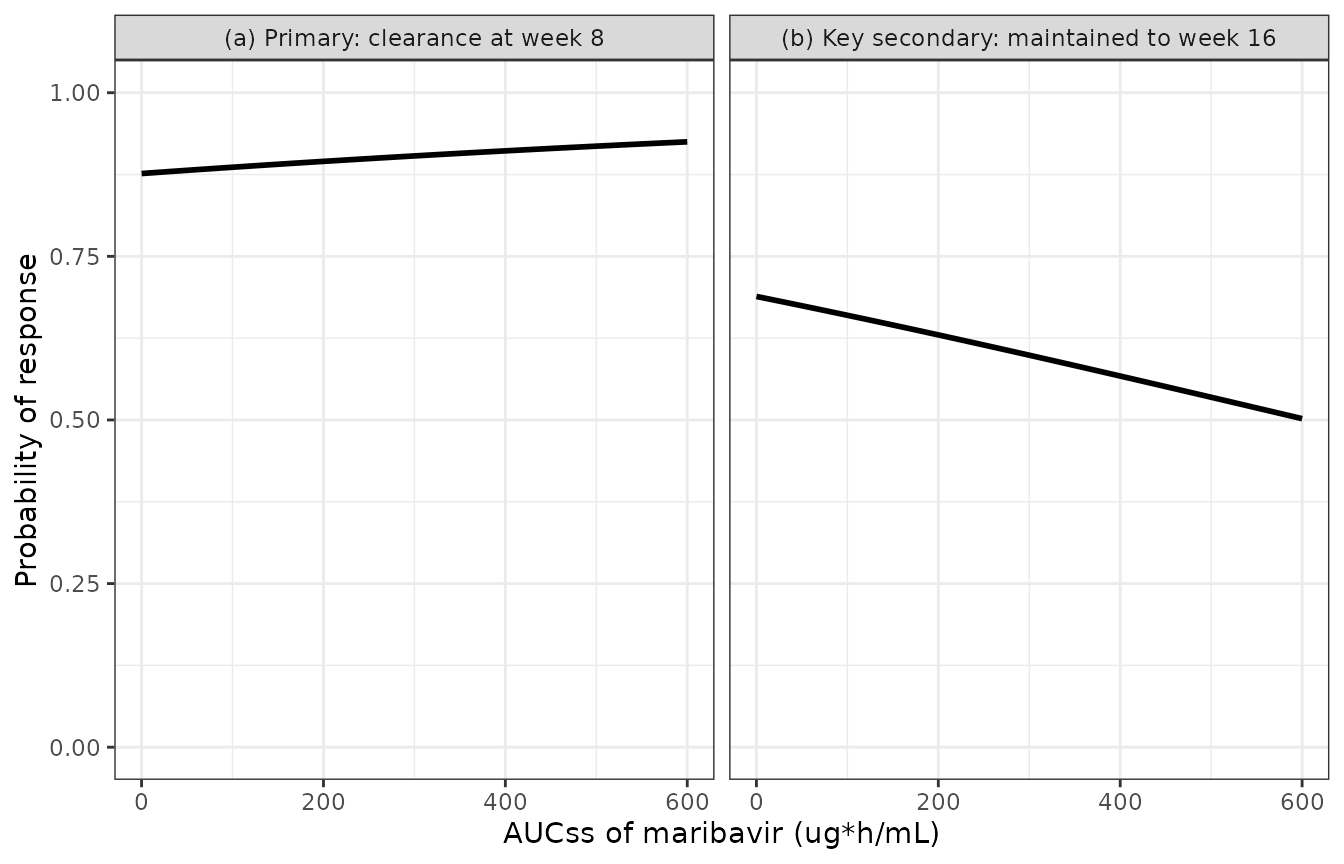
Replicates Figure 3 of Sun 2025: probability of the primary (a) and key secondary (b) endpoint as a function of steady-state maribavir AUC, for the Table S3 reference patient.
# Quantify the relationship at three exposures: zero (the intercept anchor), the
# AURORA median of roughly 170 ug*h/mL, and the top of the plotted range.
at <- function(endpoint, auc) fig3$p[fig3$Endpoint == endpoint & fig3$AUCss == auc]
eps <- unique(fig3$Endpoint)

flat <- data.frame(
  Endpoint = eps,
  `P at AUCss = 0`   = vapply(eps, at, numeric(1), auc = 0),
  `P at AUCss = 170` = vapply(eps, at, numeric(1), auc = 170),
  `P at AUCss = 600` = vapply(eps, at, numeric(1), auc = 600),
  `Odds ratio per 10 ug*h/mL` = exp(c(
    er_ini("Sun_2025_maribavir_cmv_clearance_wk8")[["e_auc_logit"]],
    er_ini("Sun_2025_maribavir_cmv_clearance_wk16")[["e_auc_logit"]])),
  `Published OR` = c(1.01, 0.987),
  check.names = FALSE, row.names = NULL
)

stopifnot(
  # Assert on the PUBLISHED quantity -- the odds ratio per 10 ug*h/mL -- rather
  # than on an absolute probability change, which depends on where each
  # intercept sits on the logistic curve and is therefore not the number the
  # paper reports. Both must round to the printed OR.
  round(flat$`Odds ratio per 10 ug*h/mL`, 2)[1] == 1.01,
  round(flat$`Odds ratio per 10 ug*h/mL`, 3)[2] == 0.987,
  # Structural: the two slopes have OPPOSITE signs. A sign error in either
  # transcription breaks this immediately.
  flat$`Odds ratio per 10 ug*h/mL`[1] > 1,
  flat$`Odds ratio per 10 ug*h/mL`[2] < 1,
  # Over the observed exposure range the movement is small in absolute terms.
  abs(flat$`P at AUCss = 170`[1] - flat$`P at AUCss = 0`[1]) < 0.05,
  abs(flat$`P at AUCss = 170`[2] - flat$`P at AUCss = 0`[2]) < 0.10
)

knitr::kable(flat, digits = 3, caption = paste(
  "Both exposure-efficacy odds ratios reproduce their published values, and",
"the two point estimates lie on opposite sides of 1."))| Endpoint | P at AUCss = 0 | P at AUCss = 170 | P at AUCss = 600 | Odds ratio per 10 ug*h/mL | Published OR |
|---|---|---|---|---|---|
| (a) Primary: clearance at week 8 | 0.877 | 0.892 | 0.925 | 1.009 | 1.010 |
| (b) Key secondary: maintained to week 16 | 0.689 | 0.639 | 0.502 | 0.987 | 0.987 |
Two things are worth reading carefully off that table, because “flat” is easy to over-claim. The odds ratios are the quantity the paper reports, and both are essentially 1 (1.01 and 0.987) with p-values of 0.503 and 0.247 – neither relationship is statistically significant, and the two point estimates fall on opposite sides of 1, which is the clearest available statement that neither carries signal.
The absolute probability movement, however, is not uniformly negligible, and the plot above shows why. The primary endpoint’s intercept of 1.96 puts its reference patient at a response probability near 0.88, out on the flat shoulder of the logistic curve, so even the full 0-600 ug*h/mL sweep moves it by under 5 percentage points. The key secondary endpoint’s intercept of 0.794 puts its reference patient near 0.69, much closer to the steep middle of the curve, so the same non-significant slope drags it down by roughly 19 percentage points across that full range – and by about 6 points across the exposures actually observed. A non-significant odds ratio is not the same thing as a visually flat probability curve, and this pair of endpoints is a clean illustration of the difference.
For contrast, the same reference-patient sweep over the safety endpoints is steeply positive for all fourteen. The two panels below place the flattest and steepest safety relationships beside each other.
safety_models <- setdiff(er_models, er_models[1:2])
aucday_grid <- seq(0, 950, by = 10)

safety_curves <- dplyr::bind_rows(lapply(safety_models, function(nm) {
  s <- solve_er(nm, "AUC_MBV_DAY", aucday_grid)
  prob_col <- grep("^prob_", names(s), value = TRUE)
  data.frame(AUCday = s$AUC_MBV_DAY, p = s[[prob_col]],
             Endpoint = sub("^Sun_2025_maribavir_", "", nm))
}))
#> Warning: multi-subject simulation without without 'omega'
#> Warning: multi-subject simulation without without 'omega'
#> Warning: multi-subject simulation without without 'omega'
#> Warning: multi-subject simulation without without 'omega'
#> Warning: multi-subject simulation without without 'omega'
#> Warning: multi-subject simulation without without 'omega'
#> Warning: multi-subject simulation without without 'omega'
#> Warning: multi-subject simulation without without 'omega'
#> Warning: multi-subject simulation without without 'omega'
#> Warning: multi-subject simulation without without 'omega'
#> Warning: multi-subject simulation without without 'omega'
#> Warning: multi-subject simulation without without 'omega'
#> Warning: multi-subject simulation without without 'omega'
#> Warning: multi-subject simulation without without 'omega'

stopifnot(
  # Every safety endpoint must be monotonically INCREASING in exposure: all
  # fourteen published slopes are positive, so a sign error anywhere breaks this.
  all(vapply(split(safety_curves, safety_curves$Endpoint),
             function(d) all(diff(d$p[order(d$AUCday)]) > 0), logical(1)))
)

ggplot2::ggplot(safety_curves, ggplot2::aes(AUCday, p, colour = Endpoint)) +
  ggplot2::geom_line(linewidth = 0.7) +
  ggplot2::coord_cartesian(ylim = c(0, 1)) +
  ggplot2::labs(x = "AUCday of maribavir (ug*h/mL)",
                y = "Probability of the adverse event", colour = NULL) +
  ggplot2::theme_bw() +
  ggplot2::theme(legend.position = "right", legend.text = ggplot2::element_text(size = 7))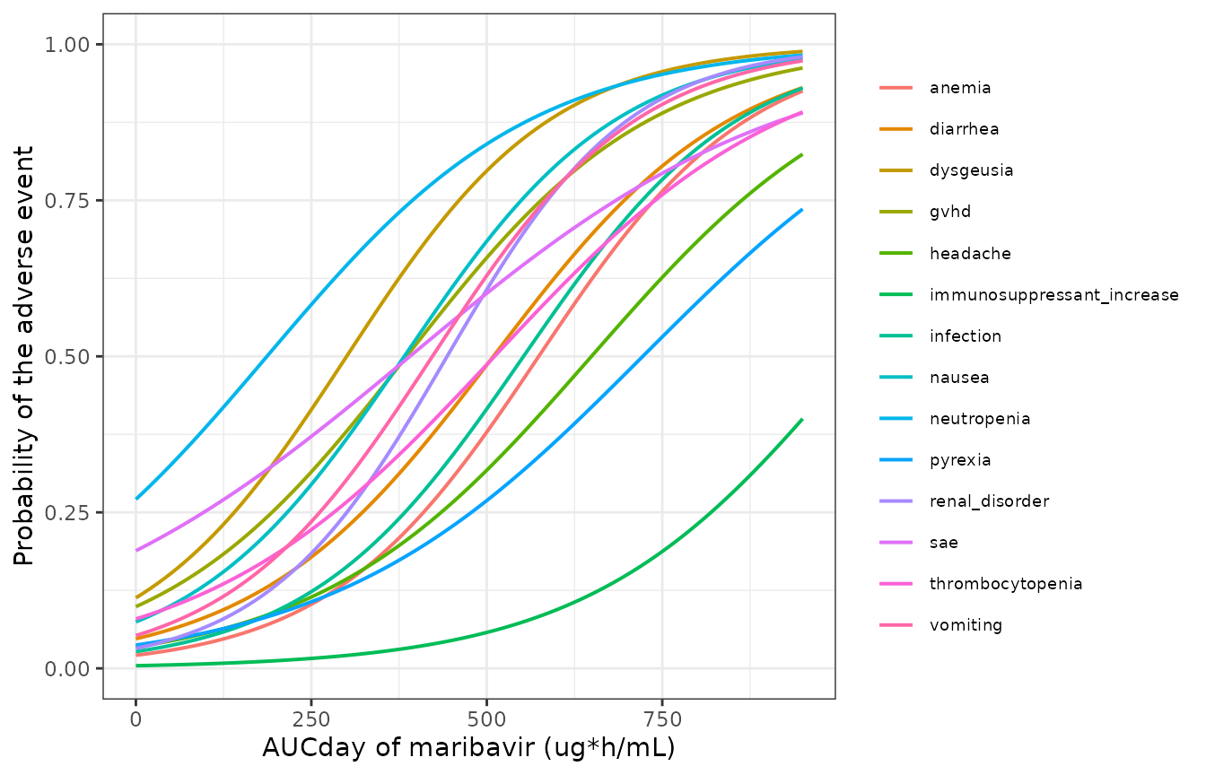
Probability of each of the fourteen treatment-emergent adverse events as a function of the day-of-event maribavir AUC, for each model’s own reference patient. Replicates the fitted curves of Figure S3.
Against the published observed quartile proportions
Figure S3 prints, for each endpoint, the observed event proportion and its 95% confidence interval within each day-of-event AUC quartile, alongside the fitted curve. Those observed proportions are a genuinely independent check on the packaged coefficients: they come from the data, not from the regression. Sun 2025 prints them for panels a and b, which are checked here.
The check has to be posed carefully. A quartile is an interval of exposures, not a point, and its top quartile is open-ended – so predicting at a midpoint would be meaningless. Instead, because each model is monotone in exposure, the predicted probability for any subject in a quartile must lie between the model’s value at that quartile’s lower and upper bound. The observed proportion is a pooled estimate over patients who differ in the model’s covariates, so the prediction is averaged over the published covariate distribution (region for dysgeusia; prior CMV prophylaxis for nausea) rather than taken at the reference stratum. The test is then whether that predicted range overlaps the observed proportion’s published confidence interval.
# Observed proportions, quartile boundaries and 95% CIs: Sun 2025 Figure S3
# panels a and b.
observed <- tibble::tribble(
  ~Endpoint,   ~lo,  ~hi, ~n_resp, ~n_tot, ~ci_lo, ~ci_hi,
  "dysgeusia", 14.1, 116,      2L,    60L,  0.004, 0.115,
  "dysgeusia", 116,  201,     10L,    59L,  0.084, 0.290,
  "dysgeusia", 201,  313,     19L,    59L,  0.206, 0.456,
  "dysgeusia", 313,  783,     30L,    60L,  0.368, 0.632,
  "nausea",      0,  116,      5L,    60L,  0.028, 0.184,
  "nausea",    116,  199,      8L,    59L,  0.060, 0.250,
  "nausea",    199,  309,     18L,    59L,  0.192, 0.439,
  "nausea",    309,  951,     33L,    60L,  0.416, 0.679
)
observed$observed <- observed$n_resp / observed$n_tot

# Published covariate distributions for the 238-patient AURORA arm (Table S2):
# region for dysgeusia, prior CMV prophylaxis for nausea. Each row is one
# stratum with its cohort weight and its covariate settings.
strata <- list(
  dysgeusia = list(
    w    = c(0.248, 0.580, 0.172),
    covs = list(list(REGION_EUROPE = 0, REGION_ASIAPACIFIC = 0),   # North America
                list(REGION_EUROPE = 1, REGION_ASIAPACIFIC = 0),   # Europe
                list(REGION_EUROPE = 0, REGION_ASIAPACIFIC = 1))), # Asia Pacific
  nausea = list(
    w    = c(0.908, 0.092),
    covs = list(list(CMV_PROPHY_PRIOR = 0), list(CMV_PROPHY_PRIOR = 1)))
)

# Cohort-weighted predicted probability at a single exposure.
pred_weighted <- function(endpoint, auc) {
  nm <- paste0("Sun_2025_maribavir_", endpoint)
  st <- strata[[endpoint]]
  ps <- vapply(st$covs, function(cv) {
    s <- solve_er(nm, "AUC_MBV_DAY", auc, extra = cv)
    s[[grep("^prob_", names(s), value = TRUE)]]
  }, numeric(1))
  sum(st$w * ps)
}

observed$pred_lo <- mapply(pred_weighted, observed$Endpoint, observed$lo)
observed$pred_hi <- mapply(pred_weighted, observed$Endpoint, observed$hi)
observed$overlaps <- observed$pred_hi >= observed$ci_lo &
                     observed$pred_lo <= observed$ci_hi

stopifnot(
  # The cohort weights must be a probability distribution.
  all(abs(vapply(strata, function(x) sum(x$w), numeric(1)) - 1) < 1e-8),
  # Monotone in exposure, so the lower bound of the predicted range really is
  # the lower bound.
  all(observed$pred_hi > observed$pred_lo),
  # The observed proportions rise monotonically across quartiles for both
  # endpoints -- the qualitative finding the figure is drawn to show.
  all(vapply(split(observed, observed$Endpoint),
             function(d) all(diff(d$observed) > 0), logical(1))),
  # Every one of the eight published quartiles must be consistent with the
  # packaged model. This is an INDEPENDENT check: the observed proportions and
  # their CIs come from the trial data, not from the regression coefficients.
  all(observed$overlaps)
)

observed |>
  dplyr::transmute(
    Endpoint,
    `AUCday quartile`   = sprintf("[%g, %g)", lo, hi),
    `Observed n/N`      = sprintf("%d/%d", n_resp, n_tot),
    `Observed (95% CI)` = sprintf("%.3f (%.3f-%.3f)", observed, ci_lo, ci_hi),
    `Predicted range`   = sprintf("%.3f-%.3f", pred_lo, pred_hi),
    Consistent          = ifelse(overlaps, "yes", "NO")
  ) |>
  knitr::kable(caption = paste(
    "Published observed event proportions per day-of-event AUC quartile",
    "(Sun 2025 Figure S3 panels a and b) against the cohort-weighted predicted",
"range from the packaged models. All eight quartiles are consistent."))| Endpoint | AUCday quartile | Observed n/N | Observed (95% CI) | Predicted range | Consistent |
|---|---|---|---|---|---|
| dysgeusia | [14.1, 116) | 2/60 | 0.033 (0.004-0.115) | 0.068-0.125 | yes |
| dysgeusia | [116, 201) | 10/59 | 0.169 (0.084-0.290) | 0.125-0.201 | yes |
| dysgeusia | [201, 313) | 19/59 | 0.322 (0.206-0.456) | 0.201-0.341 | yes |
| dysgeusia | [313, 783) | 30/60 | 0.500 (0.368-0.632) | 0.341-0.918 | yes |
| nausea | [0, 116) | 5/60 | 0.083 (0.028-0.184) | 0.068-0.135 | yes |
| nausea | [116, 199) | 8/59 | 0.136 (0.060-0.250) | 0.135-0.210 | yes |
| nausea | [199, 309) | 18/59 | 0.305 (0.192-0.439) | 0.210-0.349 | yes |
| nausea | [309, 951) | 33/60 | 0.550 (0.416-0.679) | 0.349-0.950 | yes |
End-to-end: the PK model feeds the exposure-response models
The exposure columns are not measurements. Sun 2025 derived them from the population PK model extracted above, so the two halves of the paper compose. This section closes that loop: it simulates a 400 mg twice-daily cohort with the PK model, computes each subject’s steady-state AUC by the exact mass-balance identity used earlier in this vignette, and pushes those AUCs through the primary efficacy model.
rxode2::rxSetSeed(20250911)
set.seed(20250911)

n_er  <- 200
wt_er <- pmin(pmax(stats::rlnorm(n_er, meanlog = log(73.0), sdlog = 0.23), 36.1), 141)

# 400 mg twice daily to steady state, then a dense 24 h observation window.
ev_one <- as.data.frame(
  rxode2::et(amt = 400, ii = 12, until = 24 * 20, cmt = "depot") |>
    rxode2::et(seq(24 * 19, 24 * 20, length.out = 49), cmt = "central")
)
# Keep ii / addl: dropping them would silently reduce the regimen to a
# single dose, and by hour 456 the profile would be empty.
ev_one <- ev_one[, c("time", "cmt", "amt", "ii", "addl", "evid")]

ev_er <- do.call(rbind, lapply(seq_len(n_er), function(i) {
  d <- ev_one
  d$id <- i
  d$WT <- wt_er[i]
  d
}))
ev_er$DOSE                     <- 400
ev_er$DIS_CMV                  <- 1
ev_er$CONMED_CYP3A4_INH_STRONG <- 0
ev_er$CONMED_CYP3A4_IND        <- 0
ev_er$CONMED_PPI               <- 0
ev_er$STUDY_MARIBAVIR_PHASE1   <- 0

sim_er <- rxode2::rxSolve(mod, ev_er, returnType = "data.frame", addDosing = FALSE)

# Steady-state AUC over one 12 h dosing interval: trapezoid over the final 24 h
# window, halved. At steady state the two intervals in that window are identical.
auc_tab <- sim_er |>
  dplyr::filter(!is.na(Cc)) |>
  dplyr::group_by(id) |>
  dplyr::summarise(
    AUC_MBV_SS = {
      o <- order(time)
      sum(diff(time[o]) * (utils::head(Cc[o], -1) + utils::tail(Cc[o], -1)) / 2) / 2
    },
    .groups = "drop"
  )

stopifnot(
  # The simulated exposures must land inside the range the exposure-response
  # models were fitted over. Median, not extreme, per this vignette's
  # cohort-assertion convention.
  stats::median(auc_tab$AUC_MBV_SS) > 80,
  stats::median(auc_tab$AUC_MBV_SS) < 400
)

# Push the simulated exposures through the primary efficacy model, holding the
# Table S3 reference patient in every other respect.
eff_nm <- "Sun_2025_maribavir_cmv_clearance_wk8"
eff_ev <- data.frame(id = auc_tab$id, time = 0, evid = 0L,
                     amt = NA_real_, dv = NA_real_,
                     AUC_MBV_SS = auc_tab$AUC_MBV_SS)
for (cv in setdiff(er_ui[[eff_nm]]$allCovs, "AUC_MBV_SS")) eff_ev[[cv]] <- 0
eff_sim <- rxode2::rxSolve(er_ui[[eff_nm]], eff_ev, returnType = "data.frame")
#> Warning: multi-subject simulation without without 'omega'

auc_q <- stats::quantile(auc_tab$AUC_MBV_SS, c(0.1, 0.9))
p_q   <- stats::quantile(eff_sim$prob_cmv_clearance_wk8, c(0.1, 0.9))

stopifnot(
  # The point of the exercise. A wide spread in simulated exposure must produce
  # an almost invisible spread in predicted response, because the
  # exposure-efficacy relationship is flat. If a future edit inflated the slope,
  # this bound is what catches it. Deterministic given the drawn cohort only
  # through the exposure spread, which the preceding median bounds pin.
  auc_q[[2]] / auc_q[[1]] > 1.5,
  diff(p_q) < 0.05
)

endtoend <- data.frame(
  Quantity = c("Simulated AUCss, median (ug*h/mL)",
               "Simulated AUCss, 10th-90th percentile",
               "P(clearance at week 8), median",
               "P(clearance at week 8), 10th-90th percentile"),
  Value = c(
    sprintf("%.1f", stats::median(auc_tab$AUC_MBV_SS)),
    sprintf("%.1f - %.1f", auc_q[[1]], auc_q[[2]]),
    sprintf("%.3f", stats::median(eff_sim$prob_cmv_clearance_wk8)),
    sprintf("%.3f - %.3f", p_q[[1]], p_q[[2]])
  )
)

knitr::kable(endtoend, caption = paste(
  "A", sprintf("%.1f-fold", auc_q[[2]] / auc_q[[1]]),
  "spread in simulated steady-state exposure maps to a spread of just",
  sprintf("%.3f", diff(p_q)), "in predicted probability of confirmed CMV",
  "clearance -- the paper's flat exposure-efficacy finding, reproduced",
"end to end from dose to response."))| Quantity | Value |
|---|---|
| Simulated AUCss, median (ug*h/mL) | 156.6 |
| Simulated AUCss, 10th-90th percentile | 72.0 - 282.7 |
| P(clearance at week 8), median | 0.891 |
| P(clearance at week 8), 10th-90th percentile | 0.884 - 0.902 |
Assumptions and deviations
Structural readings taken from the control stream
-
Two weight exponents rather than four. Table 2
presents four weight-effect rows, but the control stream reuses
CLWTfor Q/F andVCWTfor Vp/F, withTHETA(9)andTHETA(10)present but commentedNot used. Encoding four independent exponents would have been a silent structural error that the identical Table 2 estimates would never have exposed. -
Values from the table, structure from the code. The
control stream’s
$THETA/$OMEGA/$SIGMAblocks are initial estimates, not final ones. They are close to the published values but not equal to them (THETA(16)is-1.17initially versus a final-1.02), so none of them was used as a value.
Not published, and therefore approximated
-
The three IIV correlations. Table 2 reports only
the six IIV magnitudes; it has no correlation column and no off-diagonal
rows. The control stream shows the structure – three
$OMEGA BLOCK(2)blocks pairing CL with Vc, Q with Vp, and Ka with the lag time – and the header line;; 2. Description: 3 OMEGA BLOCKsconfirms that structure is final. This model file keeps that block structure, puts the published Table 2 variances on the diagonals, and carries the correlation coefficients (0.673, 0.820 and -0.686) from the control stream’s own$OMEGAinitial estimates, rescaled onto the published variances. These three covariances are the least well-sourced numbers in the file. They were carried rather than invented, and rather than set to zero, because the block structure is a published feature of the final model and zeroing the off-diagonals would misrepresent it; but a user who needs exact published uncertainty should treat the correlations as provisional. The magnitudes and the diagonals are unaffected. -
The
IIV (%)back-transform convention is not stated in this paper. See the Source trace section for the rule used, its provenance in the same analysis group’s companion Sun 2023 paper, and the internal-consistency check that supports it. Only Vc/F is sensitive to the choice, and only by <2% in SD.
Exposure-response models: what was and was not extracted
All sixteen fully-parameterised exposure-response regressions are
extracted, as the Sun_2025_maribavir_* family validated in
the section above. Three decisions in that extraction are deviations
worth recording.
-
Safety versus AUCss (main-paper Figure 4) is NOT extracted,
and cannot be. Nausea and vomiting show statistically
significant relationships with the STEADY-STATE metric (p = 0.0394 and
0.00296), but Figure 4 prints no coefficients – only the p-value, the
fitted curve and the observed quartile proportions. There is nothing to
transcribe, and recovering an intercept and slope by digitising a raster
figure would manufacture precision the paper never published. The
packaged
Sun_2025_maribavir_nauseaandSun_2025_maribavir_vomitingmodels are the AUCday models of Figure S3, which are a different exposure metric and a weaker causal claim: a day-of-event AUC is partly a consequence of when in the treatment course the event happened. Do not read them as the Figure 4 result. -
The headache model’s fourth T-cell-depletion level is
deliberately dropped. Figure S3 panel l reports a
Not reportedlevel with estimate-12.7and standard error1460(p = 0.993). That is the signature of complete separation – the level has exactly ONE subject in the 238-patient cohort (Table S2) – not an estimate. Shipping it would put a spuriousexp(-12.7) = 3e-6odds ratio into the model file.HCT_TCD_ALEMTUZUMAB,HCT_TCD_ATGandHCT_TCD_EXVIVOare packaged; an unreported subject falls into theNonereference. -
The anemia region coefficients follow Figure S3, not Table
S4. Table S4 assigns odds ratio 3.12 to “Europe vs. North
America” and 4.62 to “Asia Pacific vs. North America”, while Figure S3
panel j assigns 3.12 to Asia Pacific and 4.62 to Europe. The figure is
internally consistent and the table is not: the figure’s estimates
exponentiate to its own odds ratios (
exp(1.14) = 3.13for Asia Pacific,exp(1.53) = 4.62for Europe), whereas Table S4 prints odds ratios only and cannot be checked against itself. Anemia is the only endpoint where the two sources conflict.
Two further points affect how the packaged models should be consumed.
-
The exposure columns are inputs, not measurements.
Every model carries
AUC_MBV_SSorAUC_MBV_DAYas a covariate with no PK layer, exactly as the source analysis did. Derive them frommodellib("Sun_2025_maribavir"); the end-to-end section above shows the composition. -
HCT_NUCCELLhas an unstated absolute scale. Figure S3 panel m prints400 cells Referenceand a coefficient perIncrement of 1000 cells, with no multiplier and no per-kg normalisation. Read literally that is not a plausible graft cell dose – a real allogeneic graft holds on the order of 10^8 to 10^10 nucleated cells. The model file carries the source’s own numbers verbatim rather than guessing a multiplier, so it reproduces the published odds ratio whatever the underlying unit turns out to be; a user supplying a real cell dose must first rescale it onto the source’s scale. -
The placeholder residual error is not a published
quantity. Each model carries
addSd_prob_* <- fixed(0.001)purely so rxode2 has an error model to attach to the typical-value probability. The source fits a Bernoulli likelihood, which has no sigma, and estimates no random effects; the models are therefore deterministic given their covariates.
Simulation assumptions
- Weight distributions are log-normal draws matched to the Table 1 per-stratum mean and SD and truncated to the reported 36.1-141 kg range. Sun 2025 does not publish the empirical weight distribution, and Table 1 reports “NR” for the AURORA weights specifically.
- Cohort size is 200 per arm, the repository cap, against published strata of 157 and 724 individuals. The comparison is therefore of geometric means and CV%, not of individual predictions.
- Post-hoc versus prospective simulation. Table 3’s values are summaries of post-hoc Bayesian individual estimates, which are shrunk toward the typical value. This simulation draws from the full prior. Shrinkage is low for CL/F (6.9%) and moderate for Vc/F (30.8%) but high for Q/F, Vp/F and the lag time (54-56%), so the simulated CV% for trough-sensitive metrics is expected to exceed the published CV%.
- No concomitant medication in any simulated arm, matching the stated conditions for Table 3 and Figure 2. ```