BMS-986166 (Bihorel 2021)
Source:vignettes/articles/Bihorel_2021_BMS986166.Rmd
Bihorel_2021_BMS986166.RmdModel and source
Bihorel 2021 describes four models, all extracted here:
-
Bihorel_2021_BMS986166– the joint population PK model for the prodrug BMS-986166 and its active phosphorylated metabolite BMS-986166-P (Figure 1, Table 1). -
Bihorel_2021_BMS986166_nddhr– the exposure-response (E-R) model for the day-1 nadir of time-matched, placebo-corrected heart rate (nDDHR). -
Bihorel_2021_BMS986166_nalc_sdandBihorel_2021_BMS986166_nalc_md– the E-R models for the nadir absolute lymphocyte count (nALC) after a single dose and after 28 days of once-daily dosing (Table 2).
The E-R models were fitted separately, after the PK model, on
model-predicted average BMS-986166-P concentrations
(Cavg,Day1 or Cavg,Day28), so each is a
PD-only model whose exposure enters as the CAV
covariate.
- Citation: Bihorel S, Singhal S, Shevell D, Sun H, Xie J, Basdeo S, Liu A, Dutta S, Ludwig E, Huang H, Lin K, Fura A, Throup J, Girgis IG. Population Pharmacokinetic Analysis of BMS-986166, a Novel Selective Sphingosine-1-Phosphate-1 Receptor Modulator, and Exposure-Response Assessment of Lymphocyte Counts and Heart Rate in Healthy Participants. Clin Pharmacol Drug Dev. 2021;10(1):8-21. doi:10.1002/cpdd.878. PMCID: PMC7821288.
- Description (PK): Joint population PK model for BMS-986166 (an oral prodrug sphingosine-1-phosphate-1 receptor modulator) and its active phosphorylated metabolite BMS-986166-P in healthy adults (Bihorel 2021). Parent: two-compartment model with first-order absorption, linear elimination and study-specific relative bioavailability. Metabolite: one-compartment model with Michaelis-Menten elimination, fed by complete molar conversion of the parent clearance (FM = 1) plus a virtual pre-systemic BMS-986166-P dose (a fraction F2 of the molar BMS-986166 dose) delivered zero-order over D2 into a metabolite depot and then absorbed first-order. Both bioavailabilities carry study-specific fold shifts for the 12.5% of subjects the analysts identified as having low exposures. The parent PK was fitted first and then fixed while the metabolite parameters were estimated (sequential fit).
- Article: https://doi.org/10.1002/cpdd.878 (open access, PMC7821288)
Population
The analyses pooled two double-blind, placebo-controlled phase 1 studies in healthy adults, both run at one US site with a liquid oral formulation: Study IM018001 (single doses of 0.75, 2 or 5 mg; 24 active, 6 placebo) and Study IM018003 (0.25, 0.75 or 1.5 mg once daily for 28 days; 24 active, 8 placebo). Every subject received a lead-in placebo dose on day -1. The 62 participants were 96.8% male, mean age 34.7 years (19-52), mean weight 84.2 kg (58.3-104.1); 34 were White, 25 Black or African American, 2 American Indian or Alaska Native, and 1 Native Hawaiian or other Pacific Islander (Results; Supplementary Table S2 for the 48 subjects in the PK analysis).
The PK analysis used 1677 BMS-986166 and 1637 BMS-986166-P blood-lysate concentrations from the 48 actively treated subjects. The E-R analyses used 61 nDDHR values (13 from placebo recipients), 31 subjects for nALC after a single dose, and 31 for nALC after repeated dosing.
readModelDb("Bihorel_2021_BMS986166")()$population[c("n_subjects", "age_range", "weight_range", "sex_female_pct")]
#> $n_subjects
#> [1] 48
#>
#> $age_range
#> [1] "19-52 years"
#>
#> $weight_range
#> [1] "58.3-104 kg"
#>
#> $sex_female_pct
#> [1] 4.17
Source trace
Every ini() value carries an in-file comment naming its
source. They are collected here.
Joint PK model (Bihorel_2021_BMS986166)
| Parameter / equation | Value | Source location |
|---|---|---|
lka (KA) |
0.287 1/h | Table 1 |
lcl (CL) |
2.51 L/h | Table 1 |
lvc (V2) |
913 L | Table 1 |
lq (Q) |
0.763 L/h | Table 1 |
lvp (V3) |
205 L | Table 1 |
lfdepot_im018001 (F1 SAD) |
1 (fixed) | Table 1 |
lfdepot_im018003 (F1 MAD) |
0.764 | Table 1 |
e_mix_low_exposure_fdepot_im018001 (F1 SAD,LOW) |
log(0.655) | Table 1 |
e_mix_low_exposure_fdepot_im018003 (F1 MAD,LOW) |
log(0.471) | Table 1 |
fm (FM) |
1 (fixed) | Table 1 |
lvmax_bms986166p (VMAX) |
0.649 umol/h | Table 1 |
lkm_bms986166p (KM) |
0.125 uM | Table 1 |
lvc_bms986166p (VM) |
38.7 L | Table 1 |
lka_bms986166p (KAM) |
0.382 1/h | Table 1 |
ld1_bms986166p (D2) |
5.56 h | Table 1 |
lfdepot_bms986166p_im018001 (F2 SAD) |
0.0771 | Table 1 |
lfdepot_bms986166p_im018003 (F2 MAD) |
0.0797 | Table 1 |
e_mix_low_exposure_fdepot_bms986166p_im018001 (F2
SAD,LOW) |
log(1.25) | Table 1 |
e_mix_low_exposure_fdepot_bms986166p_im018003 (F2
MAD,LOW) |
log(1.82) | Table 1 |
| IIV on CL, V2, KA | 34.4, 16.8, 42.7 %CV | Table 1 |
| IIV on VMAX, VM, KAM | 34.1, 35.1, 26.1 %CV | Table 1 |
propSd, propSd_bms986166p
|
sqrt(0.00906), sqrt(0.0174) | Table 1 |
| Model structure | 2-cmt parent, 1-cmt metabolite, virtual zero-order metabolite dose | Figure 1; Results bullets |
F1 = F1study x F1study,low,
F2 = F2study x F2study,low
|
n/a | Figure 1 |
| Molecular weights 379.5 / 459.5 g/mol | n/a | PubChem (not in the paper; see Assumptions) |
Exposure-response models
| Model | Parameter | Value | Source location |
|---|---|---|---|
| nDDHR |
rbase (nDDHRplacebo) |
-9.08 bpm | Table 2 |
| nDDHR |
nadir_max (MaxDelta) |
-19.7 bpm | Table 2 |
| nDDHR |
lic50 (IC50) |
1.26 ng/mL | Table 2 |
| nDDHR |
lhill (h) |
1.84 | Table 2 |
| nDDHR | propSd |
sqrt(0.167) | Table 2 |
| nDDHR | equation | nDDHRplacebo + (MaxDelta - nDDHRplacebo) * C^h / (IC50^h + C^h) |
Results, E-R Analysis: HR |
| nALC single dose |
lrbase (ALC0), limax, lic50,
lhill, placebo_effect
|
2.061, 0.6747, 2.693 ng/mL, 3.080, 0.1992 | Table 2 |
| nALC single dose | propSd |
sqrt(0.08569) | Table 2 |
| nALC repeated dose |
lrbase (ALC0), limax, lic50,
lhill, placebo_effect
|
1.95, 0.768, 1.72 ng/mL, 1.65, 0.284 | Table 2 |
| nALC repeated dose | propSd |
sqrt(0.0880) | Table 2 |
| nALC | equation | ALC0 * (1 - Delta_placebo) * (1 - Imax * C^h / (IC50^h + C^h)) |
Results, E-R Analysis: Lymphocyte Count |
Dosing the joint PK model
The paper represents pre-systemic phosphorylation by a virtual BMS-986166-P dose: a fraction F2 of the molar BMS-986166 dose enters a metabolite depot as a zero-order input lasting D2 = 5.56 h, at the same time as the real dose. Every BMS-986166 dose therefore needs two dose records with the same mg amount:
-
cmt = "depot"– the BMS-986166 dose; -
cmt = "depot_bms986166p"withrate = -2– the virtual dose, which the model converts to umol, scales by F2 and delivers over D2.
Observation rows carry dvid = 1 (the model has two
endpoints, Cc and Cc_bms986166p, and both are
returned on every row).
# One study arm: `n` subjects, BMS-986166 `dose_mg` once daily for `n_doses`
# doses, observed on `obs_times`. Subjects are flagged as low-exposure with the
# published frequency 6/48 = 12.5%.
make_arm <- function(n, dose_mg, n_doses, obs_times, study, id_offset) {
  subj <- tibble(
    id = id_offset + seq_len(n),
    STUDY_IM018003 = as.integer(study == "IM018003"),
    MIX_LOW_EXPOSURE = rbinom(n, 1, 6 / 48)
  )
  dose_times <- 24 * (seq_len(n_doses) - 1)
  doses <- tidyr::expand_grid(subj, time = dose_times, cmt = c("depot", "depot_bms986166p")) |>
    mutate(
      amt = dose_mg, evid = 1L, dvid = NA_integer_,
      rate = if_else(cmt == "depot_bms986166p", -2, 0)
    )
  obs <- tidyr::expand_grid(subj, time = obs_times) |>
    mutate(cmt = NA_character_, amt = 0, evid = 0L, dvid = 1L, rate = 0)
  bind_rows(doses, obs) |>
    mutate(study = study, treatment = paste(study, sprintf("%g mg", dose_mg))) |>
    arrange(id, time, desc(evid))
}
Virtual cohort and stochastic simulation
Observed data are not public. The cohort mirrors the two studies’ dose groups, with 100 virtual subjects per arm. No covariate other than study and the low-exposure flag enters the PK model, so no demographic distribution is needed.
set.seed(2021)
rxode2::rxSetSeed(2021)

obs_sad <- sort(unique(c(seq(0, 48, by = 1), seq(52, 144, by = 4), seq(168, 816, by = 24))))
last_dose <- 27 * 24
obs_mad <- sort(unique(c(
  seq(0, 24, by = 1), seq(28, last_dose, by = 8),
  last_dose + seq(0, 48, by = 1), last_dose + seq(52, 144, by = 8),
  last_dose + seq(168, 1176, by = 24)
)))

n_arm <- 100L
arms <- tribble(
  ~study,     ~dose_mg, ~n_doses,
  "IM018001", 0.75,     1L,
  "IM018001", 2,        1L,
  "IM018001", 5,        1L,
  "IM018003", 0.25,     28L,
  "IM018003", 0.75,     28L,
  "IM018003", 1.5,      28L
)
events <- bind_rows(lapply(seq_len(nrow(arms)), function(i) {
  make_arm(
    n = n_arm, dose_mg = arms$dose_mg[i], n_doses = arms$n_doses[i],
    obs_times = if (arms$study[i] == "IM018001") obs_sad else obs_mad,
    study = arms$study[i], id_offset = (i - 1L) * n_arm
  )
}))
stopifnot(!anyDuplicated(unique(events[, c("id", "time", "evid", "cmt")])))
mod <- readModelDb("Bihorel_2021_BMS986166")
sim <- rxode2::rxSolve(
  mod,
  events = events,
  keep = c("study", "treatment", "MIX_LOW_EXPOSURE"),
  useLinCmt = FALSE
) |>
  as.data.frame()
#> ℹ parameter labels from comments will be replaced by 'label()'
Concentration-time profiles (Figure 3)
# Replicates the layout of Figure 3 of Bihorel 2021 (VPC by analyte and study),
# stratified here by dose group; median and 10th-90th percentiles.
sim |>
  select(id, time, study, treatment, `BMS-986166` = Cc, `BMS-986166-P` = Cc_bms986166p) |>
  pivot_longer(c(`BMS-986166`, `BMS-986166-P`), names_to = "analyte", values_to = "conc") |>
  # log axis: drop the pre-dose zeros (plotting only; PKNCA below keeps them)
  filter(conc > 0) |>
  group_by(analyte, treatment, time) |>
  summarise(
    q10 = quantile(conc, 0.10), q50 = median(conc), q90 = quantile(conc, 0.90),
    .groups = "drop"
  ) |>
  ggplot(aes(time / 24, q50, colour = treatment, fill = treatment)) +
  geom_ribbon(aes(ymin = q10, ymax = q90), alpha = 0.15, colour = NA) +
  geom_line() +
  facet_wrap(~analyte) +
  scale_y_log10() +
  labs(
    x = "Time after first dose (day)", y = "Blood concentration (ng/mL)",
    colour = NULL, fill = NULL,
    caption = "Median and 10th-90th percentiles. Compare Figure 3 of Bihorel 2021."
  ) +
  theme(legend.position = "bottom")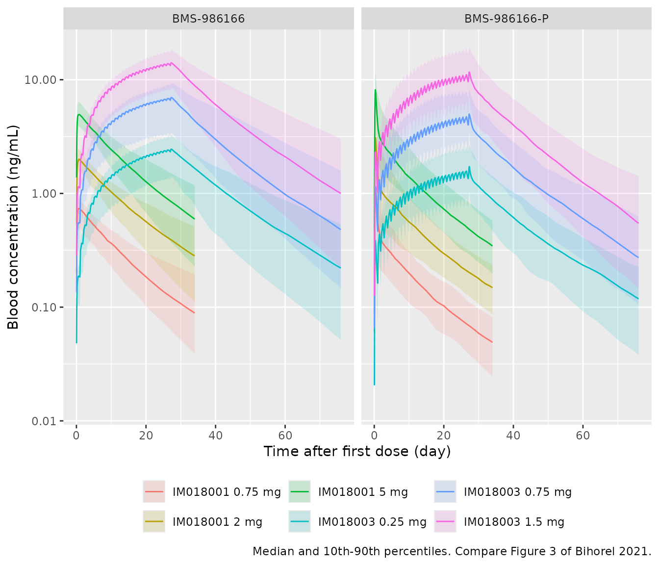
PKNCA validation
Bihorel 2021 does not tabulate NCA results, but states the following observed values: peak concentrations occurred at about 21 h (BMS-986166) and 6 h (BMS-986166-P) in Study IM018001, and at 15 h and 7.5 h in Study IM018003 (Results, Population PK Model; the IM018003 values are compared with the first dose here, because first-dose sampling in that study stopped at 15 h, Supplementary Table S1). After multiple doses, the median Tmax fell between 9 and 15 h for BMS-986166 and between 6 and 9 h for BMS-986166-P, and the apparent terminal half-life ranged from 276 to 321 h and from 270 to 304 h (Introduction, citing the clinical study report); the mid-point of each range is the reference for dose 28.
nca_one <- function(conc_col, analyte) {
  conc <- sim |>
    transmute(id, time, study, treatment, Cc = .data[[conc_col]]) |>
    filter(!is.na(Cc))
  # time-zero guarantee (pre-dose concentration is 0 for both analytes)
  conc <- bind_rows(conc, conc |> distinct(id, study, treatment) |> mutate(time = 0, Cc = 0)) |>
    distinct(id, study, treatment, time, .keep_all = TRUE) |>
    arrange(id, time)
  dose <- events |>
    filter(evid == 1, cmt == "depot") |>
    select(id, time, amt, study, treatment)
  intervals <- bind_rows(
    # single dose: whole profile, and the first 24 h for Cavg,Day1
    data.frame(start = 0, end = Inf, cmax = TRUE, tmax = TRUE, half.life = TRUE, study = "IM018001"),
    data.frame(start = 0, end = 24, cav = TRUE, study = "IM018001"),
    data.frame(start = 0, end = 24, cav = TRUE, tmax = TRUE, study = "IM018003"),
    # multiple dose: 28th dosing interval and the terminal phase after it
    data.frame(start = last_dose, end = last_dose + 24, cmax = TRUE, tmax = TRUE, cav = TRUE, study = "IM018003"),
    data.frame(start = last_dose, end = Inf, half.life = TRUE, study = "IM018003")
  ) |>
    mutate(across(c(cmax, tmax, half.life, cav), ~ coalesce(.x, FALSE)))
  res <- PKNCA::pk.nca(PKNCA::PKNCAdata(
    PKNCA::PKNCAconc(conc, Cc ~ time | study + treatment + id),
    PKNCA::PKNCAdose(dose, amt ~ time | study + treatment + id),
    intervals = intervals
  ))
  as.data.frame(res) |> mutate(analyte = analyte)
}
nca <- bind_rows(
  nca_one("Cc", "BMS-986166"),
  nca_one("Cc_bms986166p", "BMS-986166-P")
)
published <- tribble(
  ~analyte,       ~study,     ~period,   ~tmax,          ~half.life,
  "BMS-986166",   "IM018001", "dose 1",  21,             NA,
  "BMS-986166-P", "IM018001", "dose 1",  6,              NA,
  "BMS-986166",   "IM018003", "dose 1",  15,             NA,
  "BMS-986166-P", "IM018003", "dose 1",  7.5,            NA,
  "BMS-986166",   "IM018003", "dose 28", (9 + 15) / 2,   (276 + 321) / 2,
  "BMS-986166-P", "IM018003", "dose 28", (6 + 9) / 2,    (270 + 304) / 2
)
# IM018001: whole single-dose profile. IM018003: the first 24 h (Tmax only)
# and the 28th dosing interval / post-dose-28 terminal phase.
sim_cmp <- nca |>
  filter(
    PPTESTCD %in% c("tmax", "half.life"),
    (study == "IM018001" & start == 0 & is.infinite(end)) |
      (study == "IM018003" & start == 0 & PPTESTCD == "tmax") |
      (study == "IM018003" & start == last_dose)
  ) |>
  mutate(period = if_else(start == last_dose, "dose 28", "dose 1"))
cmp <- nlmixr2lib::ncaComparisonTable(
  simulated = sim_cmp,
  reference = published,
  by = c("analyte", "study", "period"),
  units = c(tmax = "h", half.life = "h"),
  tolerance_pct = 20
)
knitr::kable(cmp, caption = "Simulated (median over all dose groups) vs. published values. * differs by >20%.")| NCA parameter | analyte | study | period | Reference | Simulated | % diff |
|---|---|---|---|---|---|---|
| Tmax (h) | BMS-986166 | IM018001 | dose 1 | 21 | 15 | -28.6%* |
| Tmax (h) | BMS-986166 | IM018003 | dose 1 | 15 | 15 | +0.0% |
| Tmax (h) | BMS-986166 | IM018003 | dose 28 | 12 | 7 | -41.7%* |
| Tmax (h) | BMS-986166-P | IM018001 | dose 1 | 6 | 8 | +33.3%* |
| Tmax (h) | BMS-986166-P | IM018003 | dose 1 | 7.5 | 8 | +6.7% |
| Tmax (h) | BMS-986166-P | IM018003 | dose 28 | 7.5 | 8 | +6.7% |
| t½ (h) | BMS-986166 | IM018001 | dose 1 | — | 329 | — |
| t½ (h) | BMS-986166 | IM018003 | dose 28 | 298 | 355 | +18.9% |
| t½ (h) | BMS-986166-P | IM018001 | dose 1 | — | 327 | — |
| t½ (h) | BMS-986166-P | IM018003 | dose 28 | 287 | 353 | +23.0%* |
The simulated values are medians over every simulated dose group, the published Tmax values are observed medians read off the sampling schedule, and the dose-28 references are mid-points of ranges across dose levels, so only gross disagreement is informative here. The starred rows have three explanations:
- Single-dose Tmax (Study IM018001). Observed peaks were sampled at 3, 6, 9, 12, 15, 18 and 24 h, so an observed median is one of those grid times, whereas the simulated grid is hourly. The simulated parent Tmax of about 15 h sits between the 12-18 h samples, below the observed 21 h, and the simulated metabolite Tmax of about 8 h sits between the 6 and 9 h samples. The first-dose Tmax values in Study IM018003 agree with the observed ones, although the observed parent value there is capped by the last 15 h sample.
- Tmax after dose 28 is shorter than observed. With first-order absorption and a parent half-life of about two weeks, the within-interval peak at near steady state falls about 7 h after the dose. Bihorel 2021 reports that the peak-to-trough range grew over time in the observed data and that no model they tried captured this; the final model underpredicts individual peaks on days 14 and 28 while reproducing average exposure, which is why the paper drives the E-R models by the average concentration.
- Terminal half-life is longer than the NCA range. The Table 1 estimates give an analytic terminal half-life of about 367 h for BMS-986166 (below), and the metabolite, whose formation is rate-limiting, follows the parent. The NCA half-lives of 270-321 h come from observed data truncated at 816 h or 1176 h after the last dose.
Typical-value checks against the paper’s statements
The Discussion states that a Cavg,Day28 of 3.5 ng/mL “typically corresponds to a BMS-986166 dose of 0.5 mg/day”, and that at this dose the typical nDDHR on day 1 is -11.0 bpm against -9.1 bpm for placebo. Both claims are checked on typical-value solves (no IIV) of a normal-exposure subject in Study IM018003.
mod_typical <- rxode2::zeroRe(mod)
#> ℹ parameter labels from comments will be replaced by 'label()'
cavg_typical <- function(dose_mg, study = "IM018003", low = 0L) {
  ev <- make_arm(
    n = 1L, dose_mg = dose_mg, n_doses = 28L,
    obs_times = sort(unique(c(seq(0, 24, by = 0.25), last_dose + seq(0, 24, by = 0.25)))),
    study = study, id_offset = 0L
  ) |>
    mutate(MIX_LOW_EXPOSURE = low)
  s <- rxode2::rxSolve(mod_typical, events = ev, useLinCmt = FALSE) |> as.data.frame()
  auc24 <- function(t, c) sum(diff(t) * (head(c, -1) + tail(c, -1)) / 2) / 24
  d1 <- s[s$time <= 24, ]
  d28 <- s[s$time >= last_dose & s$time <= last_dose + 24, ]
  c(
    day1 = auc24(d1$time, d1$Cc_bms986166p),
    day28 = auc24(d28$time, d28$Cc_bms986166p)
  )
}
cav_05 <- cavg_typical(0.5)
#> ℹ omega/sigma items treated as zero: 'etalcl', 'etalvc', 'etalka', 'etalvmax_bms986166p', 'etalvc_bms986166p', 'etalka_bms986166p'
cav_05
#>      day1     day28
#> 0.4904191 3.4645167
mod_hr <- readModelDb("Bihorel_2021_BMS986166_nddhr")
mod_sd <- readModelDb("Bihorel_2021_BMS986166_nalc_sd")
mod_md <- readModelDb("Bihorel_2021_BMS986166_nalc_md")

# Typical E-R predictions for a vector of exposures (no residual error)
er_typical <- function(mod_er, cav, outcome) {
  ev <- data.frame(id = seq_along(cav), time = 0, evid = 0L, amt = 0, CAV = cav)
  rxode2::rxSolve(rxode2::zeroRe(mod_er), events = ev, keep = "CAV") |>
    as.data.frame() |>
    pull(outcome)
}
nddhr_05 <- er_typical(mod_hr, c(0, cav_05[["day1"]]), "nadir_hr_change")
#> Warning: No omega parameters in the model
#> Warning: multi-subject simulation without without 'omega'
nalc_05 <- er_typical(mod_md, c(0, cav_05[["day28"]]), "nadir_lymphocyte_count")
#> Warning: No omega parameters in the model
#> multi-subject simulation without without 'omega'

checks <- tibble(
  Quantity = c(
    "Cavg,Day28 at 0.5 mg/day (ng/mL)",
    "nDDHR, placebo (bpm)",
    "nDDHR, day 1 of 0.5 mg/day (bpm)",
    "Maximal drug effect on nDDHR (bpm)"
  ),
  Paper = c(3.5, -9.1, -11.0, -10.6),
  Model = c(cav_05[["day28"]], nddhr_05[1], nddhr_05[2], -19.7 - (-9.08))
) |>
  mutate(`% diff` = round(100 * (Model / Paper - 1), 1))
knitr::kable(checks, digits = 2, caption = "Typical-value checks against Bihorel 2021 Discussion.")| Quantity | Paper | Model | % diff |
|---|---|---|---|
| Cavg,Day28 at 0.5 mg/day (ng/mL) | 3.5 | 3.46 | -1.0 |
| nDDHR, placebo (bpm) | -9.1 | -9.08 | -0.2 |
| nDDHR, day 1 of 0.5 mg/day (bpm) | -11.0 | -10.67 | -3.0 |
| Maximal drug effect on nDDHR (bpm) | -10.6 | -10.62 | 0.2 |
stopifnot(
  # A wrong molecular weight, molar conversion or F2 moves Cavg,Day28 by far more.
  abs(cav_05[["day28"]] / 3.5 - 1) < 0.05,
  abs(nddhr_05[1] / -9.08 - 1) < 1e-6,
  abs(nddhr_05[2] / -11.0 - 1) < 0.05
)
The same solve gives a typical nALC at 0.5 mg/day of 0.581 x 10^3 cells/uL, a 58.4% reduction relative to placebo and a 70.2% reduction from ALC0. The paper’s Discussion and Conclusion attribute a “65% reduction” to this dose, which neither reading reproduces exactly; see Assumptions and deviations.
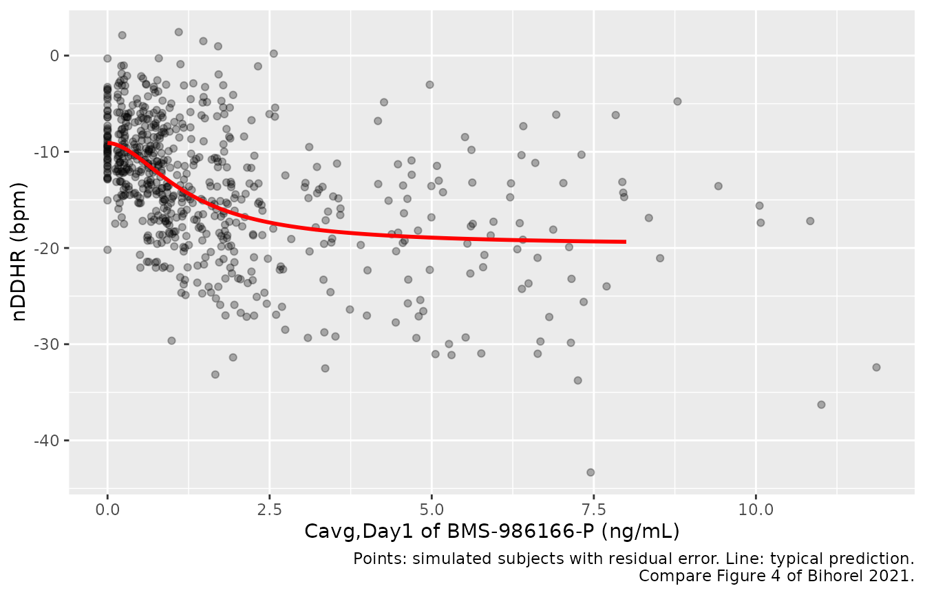
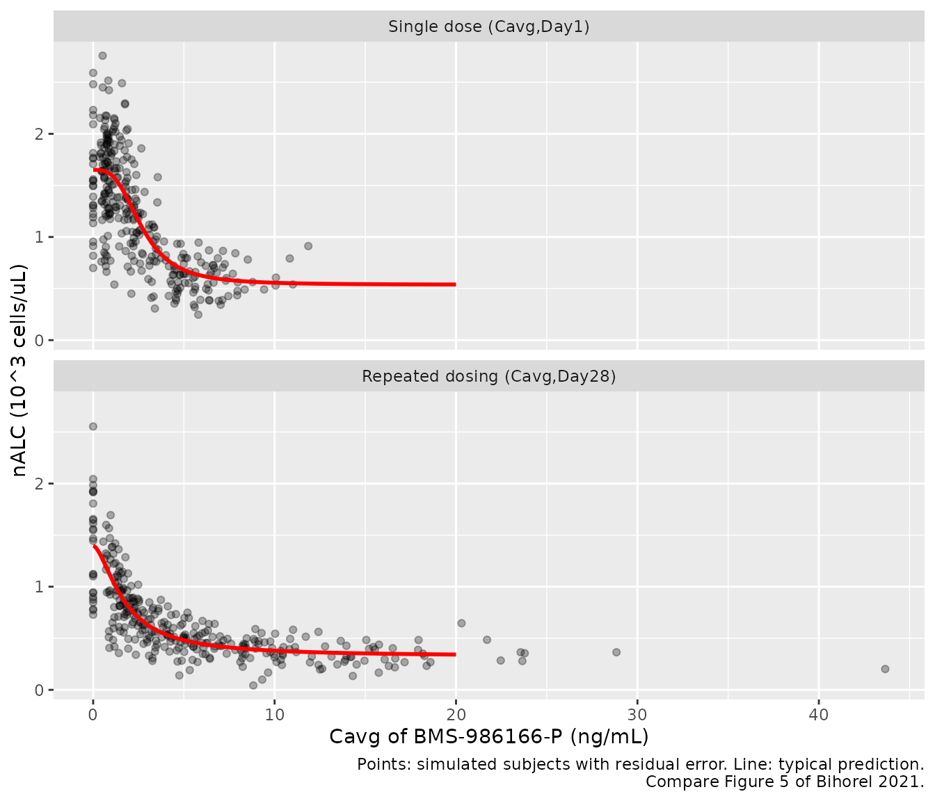
Exposure-response models (Figures 4 and 5)
The E-R models take one exposure per subject. Here the individual
Cavg,Day1 and Cavg,Day28 of the simulated PK cohort feed them directly,
which is the same two-stage procedure the paper used (individual PK
predictions, then E-R). Placebo recipients have CAV = 0; 25
virtual placebo subjects are added per study.
cav_ind <- nca |>
  filter(PPTESTCD == "cav", analyte == "BMS-986166-P") |>
  mutate(window = if_else(start == 0, "day1", "day28")) |>
  select(id, study, treatment, window, PPORRES) |>
  pivot_wider(names_from = window, values_from = PPORRES)

placebo <- tibble(
  id = max(cav_ind$id) + seq_len(50),
  study = rep(c("IM018001", "IM018003"), each = 25),
  treatment = paste(study, "placebo"), day1 = 0, day28 = 0
)
er_subj <- bind_rows(cav_ind, placebo)

solve_er <- function(mod_er, cav, subj) {
  ev <- subj |>
    transmute(id, time = 0, evid = 0L, amt = 0, CAV = .data[[cav]], treatment)
  rxode2::rxSolve(mod_er, events = ev, keep = c("CAV", "treatment")) |> as.data.frame()
}
sim_hr <- solve_er(mod_hr, "day1", er_subj)
#> Warning: multi-subject simulation without without 'omega'
sim_sd <- solve_er(mod_sd, "day1", filter(er_subj, study == "IM018001"))
#> Warning: multi-subject simulation without without 'omega'
sim_md <- solve_er(mod_md, "day28", filter(er_subj, study == "IM018003"))
#> Warning: multi-subject simulation without without 'omega'
# Replicates Figure 4 of Bihorel 2021: nDDHR vs model-predicted Cavg,Day1.
curve_c <- seq(0, 8, by = 0.05)
curve_hr <- tibble(CAV = curve_c, pred = er_typical(mod_hr, curve_c, "nadir_hr_change"))
#> Warning: No omega parameters in the model
#> Warning: multi-subject simulation without without 'omega'
ggplot(sim_hr, aes(CAV, sim)) +
  geom_point(alpha = 0.3) +
  geom_line(data = curve_hr, aes(CAV, pred), colour = "red", linewidth = 1) +
  labs(
    x = "Cavg,Day1 of BMS-986166-P (ng/mL)", y = "nDDHR (bpm)",
    caption = "Points: simulated subjects with residual error. Line: typical prediction.\nCompare Figure 4 of Bihorel 2021."
  )
# Replicates Figure 5 of Bihorel 2021: nALC vs Cavg after single (top) and
# repeated (bottom) dosing.
curve_c2 <- seq(0, 20, by = 0.05)
curves <- bind_rows(
  tibble(model = "Single dose (Cavg,Day1)", CAV = curve_c2, pred = er_typical(mod_sd, curve_c2, "nadir_lymphocyte_count")),
  tibble(model = "Repeated dosing (Cavg,Day28)", CAV = curve_c2, pred = er_typical(mod_md, curve_c2, "nadir_lymphocyte_count"))
)
#> Warning: No omega parameters in the model
#> Warning: multi-subject simulation without without 'omega'
#> Warning: No omega parameters in the model
#> Warning: multi-subject simulation without without 'omega'
pts <- bind_rows(
  sim_sd |> mutate(model = "Single dose (Cavg,Day1)"),
  sim_md |> mutate(model = "Repeated dosing (Cavg,Day28)")
)
ggplot(pts, aes(CAV, sim)) +
  geom_point(alpha = 0.3) +
  geom_line(data = curves, aes(CAV, pred), colour = "red", linewidth = 1) +
  facet_wrap(~ factor(model, levels = unique(curves$model)), ncol = 1) +
  labs(
    x = "Cavg of BMS-986166-P (ng/mL)", y = "nALC (10^3 cells/uL)",
    caption = "Points: simulated subjects with residual error. Line: typical prediction.\nCompare Figure 5 of Bihorel 2021."
  )
The abstract summarises the E-R fits as 9 bpm and 20% decreases in nDDHR and nALC with placebo, a maximal drug effect of 10 bpm on nDDHR, and about 80% maximal reduction of nALC from drug and placebo together. The typical values of the extracted models reproduce these directly (the 20% placebo figure matches the single-dose model; the repeated-dose model’s Table 2 estimate is 28.4%, which the Discussion attributes to selection bias among the few placebo recipients):
limits <- tibble(
  Quantity = c(
    "nDDHR, placebo (bpm)", "Maximal drug effect on nDDHR (bpm)",
    "nALC reduction from ALC0, placebo, single dose (%)",
    "Maximal nALC reduction from ALC0, repeated dosing (%)"
  ),
  Paper = c(-9, -10, 20, 80),
  Model = c(
    er_typical(mod_hr, 0, "nadir_hr_change"),
    er_typical(mod_hr, 1e4, "nadir_hr_change") - er_typical(mod_hr, 0, "nadir_hr_change"),
    100 * (1 - er_typical(mod_sd, 0, "nadir_lymphocyte_count") / 2.061),
    100 * (1 - er_typical(mod_md, 1e4, "nadir_lymphocyte_count") / 1.95)
  )
)
#> Warning: No omega parameters in the model
#> No omega parameters in the model
#> No omega parameters in the model
#> No omega parameters in the model
#> No omega parameters in the model
knitr::kable(limits, digits = 1, caption = "Rounded E-R summaries in the Bihorel 2021 abstract.")| Quantity | Paper | Model |
|---|---|---|
| nDDHR, placebo (bpm) | -9 | -9.1 |
| Maximal drug effect on nDDHR (bpm) | -10 | -10.6 |
| nALC reduction from ALC0, placebo, single dose (%) | 20 | 19.9 |
| Maximal nALC reduction from ALC0, repeated dosing (%) | 80 | 83.4 |
Dose-response simulation (Figure 6)
Figure 6 of Bihorel 2021 shows typical changes relative to placebo in nDDHR on day 1 and in nALC after 28 days of dosing, against the daily dose, for subjects with normal and with low exposures. The paper does not say which study’s bioavailability its simulations used for the lymphocyte endpoint; Study IM018003 is used here because the repeated-dose nALC model belongs to it.
doses <- c(0.1, 0.25, 0.5, 0.75, 1, 1.5, 2, 3, 4, 5)
dr <- tidyr::expand_grid(dose = doses, low = c(0L, 1L))
dr$cav <- lapply(seq_len(nrow(dr)), function(i) cavg_typical(dr$dose[i], low = dr$low[i]))
#> ℹ omega/sigma items treated as zero: 'etalcl', 'etalvc', 'etalka', 'etalvmax_bms986166p', 'etalvc_bms986166p', 'etalka_bms986166p'
#> ℹ omega/sigma items treated as zero: 'etalcl', 'etalvc', 'etalka', 'etalvmax_bms986166p', 'etalvc_bms986166p', 'etalka_bms986166p'
#> ℹ omega/sigma items treated as zero: 'etalcl', 'etalvc', 'etalka', 'etalvmax_bms986166p', 'etalvc_bms986166p', 'etalka_bms986166p'
#> ℹ omega/sigma items treated as zero: 'etalcl', 'etalvc', 'etalka', 'etalvmax_bms986166p', 'etalvc_bms986166p', 'etalka_bms986166p'
#> ℹ omega/sigma items treated as zero: 'etalcl', 'etalvc', 'etalka', 'etalvmax_bms986166p', 'etalvc_bms986166p', 'etalka_bms986166p'
#> ℹ omega/sigma items treated as zero: 'etalcl', 'etalvc', 'etalka', 'etalvmax_bms986166p', 'etalvc_bms986166p', 'etalka_bms986166p'
#> ℹ omega/sigma items treated as zero: 'etalcl', 'etalvc', 'etalka', 'etalvmax_bms986166p', 'etalvc_bms986166p', 'etalka_bms986166p'
#> ℹ omega/sigma items treated as zero: 'etalcl', 'etalvc', 'etalka', 'etalvmax_bms986166p', 'etalvc_bms986166p', 'etalka_bms986166p'
#> ℹ omega/sigma items treated as zero: 'etalcl', 'etalvc', 'etalka', 'etalvmax_bms986166p', 'etalvc_bms986166p', 'etalka_bms986166p'
#> ℹ omega/sigma items treated as zero: 'etalcl', 'etalvc', 'etalka', 'etalvmax_bms986166p', 'etalvc_bms986166p', 'etalka_bms986166p'
#> ℹ omega/sigma items treated as zero: 'etalcl', 'etalvc', 'etalka', 'etalvmax_bms986166p', 'etalvc_bms986166p', 'etalka_bms986166p'
#> ℹ omega/sigma items treated as zero: 'etalcl', 'etalvc', 'etalka', 'etalvmax_bms986166p', 'etalvc_bms986166p', 'etalka_bms986166p'
#> ℹ omega/sigma items treated as zero: 'etalcl', 'etalvc', 'etalka', 'etalvmax_bms986166p', 'etalvc_bms986166p', 'etalka_bms986166p'
#> ℹ omega/sigma items treated as zero: 'etalcl', 'etalvc', 'etalka', 'etalvmax_bms986166p', 'etalvc_bms986166p', 'etalka_bms986166p'
#> ℹ omega/sigma items treated as zero: 'etalcl', 'etalvc', 'etalka', 'etalvmax_bms986166p', 'etalvc_bms986166p', 'etalka_bms986166p'
#> ℹ omega/sigma items treated as zero: 'etalcl', 'etalvc', 'etalka', 'etalvmax_bms986166p', 'etalvc_bms986166p', 'etalka_bms986166p'
#> ℹ omega/sigma items treated as zero: 'etalcl', 'etalvc', 'etalka', 'etalvmax_bms986166p', 'etalvc_bms986166p', 'etalka_bms986166p'
#> ℹ omega/sigma items treated as zero: 'etalcl', 'etalvc', 'etalka', 'etalvmax_bms986166p', 'etalvc_bms986166p', 'etalka_bms986166p'
#> ℹ omega/sigma items treated as zero: 'etalcl', 'etalvc', 'etalka', 'etalvmax_bms986166p', 'etalvc_bms986166p', 'etalka_bms986166p'
#> ℹ omega/sigma items treated as zero: 'etalcl', 'etalvc', 'etalka', 'etalvmax_bms986166p', 'etalvc_bms986166p', 'etalka_bms986166p'
dr <- dr |>
  mutate(day1 = vapply(cav, `[[`, numeric(1), "day1"), day28 = vapply(cav, `[[`, numeric(1), "day28")) |>
  select(-cav)
hr_pbo <- er_typical(mod_hr, 0, "nadir_hr_change")
#> Warning: No omega parameters in the model
alc_pbo <- er_typical(mod_md, 0, "nadir_lymphocyte_count")
#> Warning: No omega parameters in the model
dr <- dr |>
  mutate(
    `Change in nDDHR vs placebo (bpm)` = er_typical(mod_hr, day1, "nadir_hr_change") - hr_pbo,
    `Change in nALC vs placebo (%)` = 100 * (er_typical(mod_md, day28, "nadir_lymphocyte_count") / alc_pbo - 1),
    exposure = if_else(low == 1L, "Low exposure", "Normal exposure")
  )
#> Warning: There were 4 warnings in `mutate()`.
#> The first warning was:
#> ℹ In argument: `Change in nDDHR vs placebo (bpm) = er_typical(mod_hr, day1,
#>   "nadir_hr_change") - hr_pbo`.
#> Caused by warning:
#> ! No omega parameters in the model
#> ℹ Run `dplyr::last_dplyr_warnings()` to see the 3 remaining warnings.
dr |>
  pivot_longer(starts_with("Change"), names_to = "endpoint", values_to = "value") |>
  ggplot(aes(dose, value, colour = exposure)) +
  geom_line() +
  geom_point() +
  facet_wrap(~endpoint, scales = "free_y", ncol = 1) +
  labs(
    x = "BMS-986166 dose (mg/day)", y = NULL, colour = NULL,
    caption = "Typical values, Study IM018003 bioavailability. Compare Figure 6 of Bihorel 2021."
  ) +
  theme(legend.position = "bottom")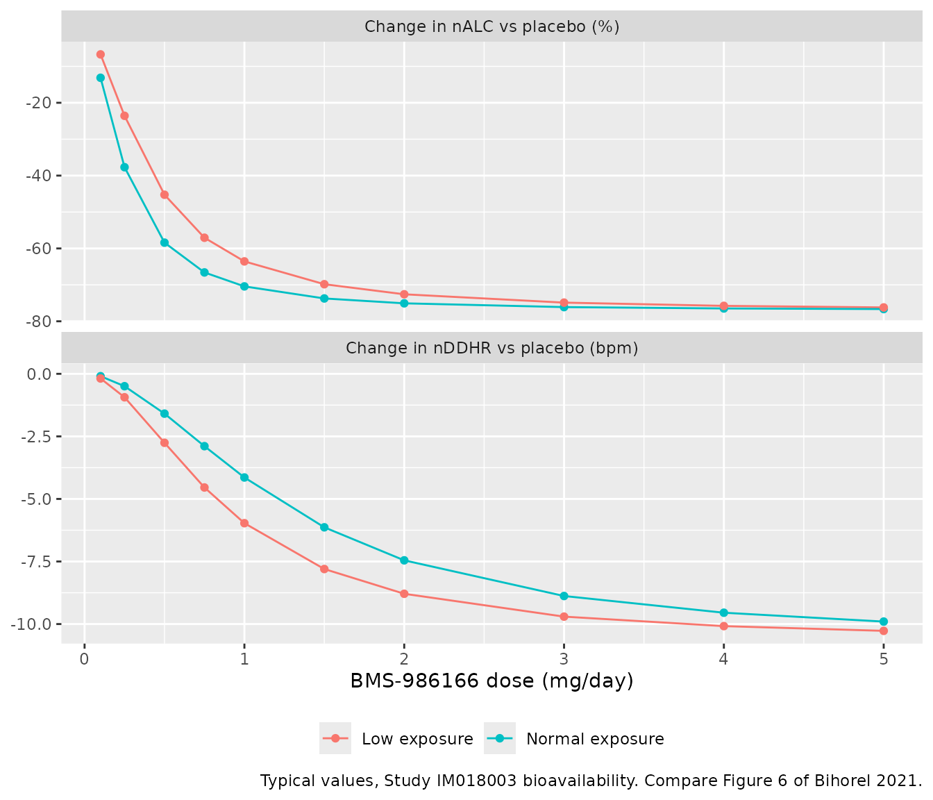
dr |>
  select(exposure, dose, day1, day28, starts_with("Change")) |>
  rename("Exposure class" = exposure, "Dose (mg/day)" = dose, "Cavg,Day1 (ng/mL)" = day1, "Cavg,Day28 (ng/mL)" = day28) |>
knitr::kable(digits = 2, caption = "Typical Cavg and E-R predictions by dose.")| Exposure class | Dose (mg/day) | Cavg,Day1 (ng/mL) | Cavg,Day28 (ng/mL) | Change in nDDHR vs placebo (bpm) | Change in nALC vs placebo (%) |
|---|---|---|---|---|---|
| Normal exposure | 0.10 | 0.10 | 0.66 | -0.09 | -13.14 |
| Low exposure | 0.10 | 0.14 | 0.42 | -0.19 | -6.72 |
| Normal exposure | 0.25 | 0.24 | 1.68 | -0.49 | -37.69 |
| Low exposure | 0.25 | 0.35 | 1.05 | -0.94 | -23.58 |
| Normal exposure | 0.50 | 0.49 | 3.46 | -1.59 | -58.41 |
| Low exposure | 0.50 | 0.71 | 2.14 | -2.76 | -45.25 |
| Normal exposure | 0.75 | 0.74 | 5.36 | -2.89 | -66.58 |
| Low exposure | 0.75 | 1.08 | 3.27 | -4.54 | -57.06 |
| Normal exposure | 1.00 | 0.99 | 7.37 | -4.14 | -70.42 |
| Low exposure | 1.00 | 1.44 | 4.45 | -5.97 | -63.55 |
| Normal exposure | 1.50 | 1.49 | 11.80 | -6.13 | -73.73 |
| Low exposure | 1.50 | 2.19 | 6.95 | -7.80 | -69.82 |
| Normal exposure | 2.00 | 2.01 | 16.88 | -7.45 | -75.07 |
| Low exposure | 2.00 | 2.96 | 9.65 | -8.79 | -72.59 |
| Normal exposure | 3.00 | 3.05 | 29.57 | -8.88 | -76.10 |
| Low exposure | 3.00 | 4.54 | 15.80 | -9.70 | -74.87 |
| Normal exposure | 4.00 | 4.13 | 47.24 | -9.55 | -76.48 |
| Low exposure | 4.00 | 6.20 | 23.17 | -10.08 | -75.76 |
| Normal exposure | 5.00 | 5.24 | 73.12 | -9.90 | -76.64 |
| Low exposure | 5.00 | 7.93 | 32.14 | -10.27 | -76.19 |
For normal-exposure subjects the paper places the 65% reduction in nALC relative to placebo at 0.75-2 mg/day, with an nDDHR change of at most -8 bpm relative to placebo, and at 1-1.75 mg/day for low-exposure subjects. Those ranges are read from the 90% confidence bands of Figure 6; the typical curves above cross -65% near the lower end of each range.
# Dose at which the typical nALC change vs placebo first reaches -65%
dose_65 <- dr |>
  group_by(exposure) |>
  summarise(dose = min(dose[`Change in nALC vs placebo (%)` <= -65]), .groups = "drop")
dose_65
#> # A tibble: 2 × 2
#>   exposure         dose
#>   <chr>           <dbl>
#> 1 Low exposure     1.5
#> 2 Normal exposure  0.75
stopifnot(
  # Deterministic typical-value solves, so the bounds are the paper's ranges
  # widened by one step of the dose grid on the low side.
  dose_65$dose[dose_65$exposure == "Normal exposure"] <= 2,
  dose_65$dose[dose_65$exposure == "Normal exposure"] >= 0.5,
  dose_65$dose[dose_65$exposure == "Low exposure"] <= 1.75,
  dose_65$dose[dose_65$exposure == "Low exposure"] >= 0.75,
  # nDDHR change vs placebo at 2 mg/day, normal exposure: about -8 bpm
  abs(dr$`Change in nDDHR vs placebo (bpm)`[dr$dose == 2 & dr$low == 0L] / -8 - 1) < 0.15
)
Assumptions and deviations
- Molecular weights are not from the paper. The model is molar (VMAX in umol/h, KM in uM, a virtual dose “equal to the molar amounts of BMS-986166 doses”), while doses are in mg and concentrations in ng/mL, so both molecular weights are required but unprinted. The maintainers took them from PubChem (CID 118877516): BMS-986166 C25H33NO2, 379.5 g/mol, and the phosphate ester BMS-986166-P C25H34NO5P, 459.5 g/mol. The 80.0 g/mol difference is the HPO3 of a phosphate ester, and the shared m/z 345 product ion the assay monitored for both analytes is consistent with these formulas. The Discussion anchor “Cavg,Day28 of 3.5 ng/mL … 0.5 mg/day” is reproduced to within 1%, which a wrong molecular weight would not allow.
- IIV scale. Table 1 reports IIV as %CV of exponential models without the variance. The maintainers converted with omega^2 = log(1 + CV^2). The residual magnitudes are reported with both variance and %CV, and there %CV = 100 * sqrt(variance); using omega^2 = CV^2 for the IIV instead would change the variances by 1-8%.
- Residual error form. The paper tested additive, constant-CV and logarithmic residual models without saying which were retained; each reported residual is a single variance, encoded here as a proportional (constant-CV) error with SD = sqrt(variance). For the negative-valued nDDHR endpoint a log-scale error is impossible, which supports the constant-CV reading.
-
Low-exposure class. Six of the 48 subjects were
flagged as low-exposure subjects by visual inspection before the fit,
with study-specific fold changes on F1 and F2. The flag is carried as
the covariate
MIX_LOW_EXPOSURE; the virtual cohort draws it with probability 6/48. -
Sequential fit. The parent parameters were
estimated first and then fixed while the metabolite parameters were
estimated. They are left as estimated (not
fixed()) values inini(), since they are the parent fit’s estimates. - No IIV correlation. The paper reports no off-diagonal IIV elements; the matrix is diagonal.
- nALC at 0.5 mg/day. The Abstract, Discussion and Conclusion associate 0.5 mg/day with a 65% reduction in nALC. The typical model gives about 58% relative to placebo and about 70% from ALC0 at the Cavg,Day28 of 3.5 ng/mL that the same Discussion sentence names. No parameter was adjusted; the statement is likely taken from the uncertainty-based simulations of Figure 6 rather than the typical-value curve.
- Tmax after repeated dosing and terminal half-life. The model’s near-steady-state Tmax (about 7 h) is shorter, and its terminal half-life (about 360 h) longer, than the published NCA summaries. Both follow from the Table 1 estimates as printed and from the misfit of peak concentrations on days 14 and 28 that the paper itself reports; no parameter was adjusted.
- E-R exposures. The paper’s E-R models were fitted to model-predicted (MAP Bayesian) Cavg. The vignette feeds them the Cavg of simulated subjects, which include IIV but no residual error, the analogue of that procedure.
- Literature check. No erratum or correction notice for Bihorel 2021 was found in PubMed or Europe PMC as of 2026-09-30.