Tocilizumab (Bastida 2018)
Source:vignettes/articles/Bastida_2018_tocilizumab.Rmd
Bastida_2018_tocilizumab.RmdModel and source
- Citation: Bastida C, Ruiz-Esquide V, Pascal M, de Vries Schultink AHM, Yague J, Sanmarti R, Huitema ADR, Soy D. Fixed dosing of intravenous tocilizumab in rheumatoid arthritis. Results from a population pharmacokinetic analysis. Br J Clin Pharmacol. 2018;84(4):716-725. doi:10.1111/bcp.13500
- Description: One-compartment population PK model for intravenous tocilizumab in adults with rheumatoid arthritis (Bastida 2018), with parallel first-order linear and Michaelis-Menten elimination from the central compartment; total body weight and time-varying C-reactive protein on linear CL.
- Article: Br J Clin Pharmacol. 2018;84(4):716-725
Population
Bastida 2018 is a single-center, prospective, observational study of 35 adults (31, 88.6%, women) with rheumatoid arthritis (RA) treated with intravenous tocilizumab at the Hospital Clinic of Barcelona (Bastida 2018 Methods, p717; Results, p718). The cohort received treatment with a 1-hour IV infusion of tocilizumab at 4, 6, or 8 mg/kg every 28 days, chosen at the rheumatologist’s discretion (54% received the 8 mg/kg regimen, 23% each the 6 and 4 mg/kg regimens). A total of 109 serum tocilizumab samples were drawn: 54 trough concentrations and 55 intermediate samples taken approximately 7, 14, and 21 days after an infusion. 16/35 patients contributed a single sample; the remaining 19 contributed an average of 5 samples each.
Baseline demographics (Bastida 2018 Table 1, p718): mean age 54.1 +/- 12.3 years, mean weight 63.5 +/- 13.8 kg, mean height 161 +/- 8.1 cm, mean CRP 0.29 +/- 0.76 mg/dL. Ethnicity: 80% White/Caucasian, 17.1% Hispanic, 2.9% Afro-American. 74% of patients were in DAS28 remission at inclusion, with 11% low and 14% moderate disease activity; 82.9% had erosive RA. Anti-drug antibodies were tested in all samples with tocilizumab < 1 ug/mL (n = 17) and were not detected in any sample.
The same information is available programmatically via
readModelDb("Bastida_2018_tocilizumab")$population.
Source trace
Every structural parameter, covariate effect, IIV element, and residual-error term below is taken from Bastida 2018 Table 2 (p720). The closed-form covariate equation for linear CL is given in the Results section (p719):
CL = 0.0104 * (WT/62)^0.360 * (1 + 0.131 * (CRP - 0.484))
where WT is total body weight in kg, CRP is C-reactive protein in mg/dL (the paper uses the Spanish abbreviation PCR for CRP in the equation), the reference weight is 62 kg and the reference CRP is 0.484 mg/dL.
| Equation / parameter | Value | Source location |
|---|---|---|
lcl (linear CL) |
log(0.0104) L/h |
Table 2, “CL, l h-1” row |
lvc (V) |
log(4.83) L |
Table 2, “V, l” row |
lvmax (Vmax) |
log(0.239) mg/h |
Table 2, “VM, mg h-1” row |
lkm (Km) |
log(4.22) ug/mL |
Table 2, “KM, ug ml-1” row |
e_wt_cl (WT/62 exponent on linear CL) |
0.360 |
Table 2, “WT(kg) on CL”; equation p719 |
e_crp_cl (linear coef on CRP - 0.484) |
0.131 1/(mg/dL) |
Table 2, “CRP (mg dL-1) on CL”; equation p719 |
var(etalcl) |
log(1 + 0.170^2) = 0.0285 |
Table 2 IIV section, CL CV 17.0% |
var(etalvc) |
log(1 + 0.308^2) = 0.0907 |
Table 2 IIV section, V CV 30.8% |
propSd |
0.255 |
Table 2 “Proportional” row, 25.5% |
addSd |
0.161 ug/mL |
Table 2 “Additive” row, 0.161 ug/mL |
| Structure (1-cmt + parallel linear + MM elimination from central) | n/a | Methods p717-718; Results p719; equation p719 |
Parameterization notes
-
One-compartment IV with parallel linear and Michaelis-Menten
elimination. Bastida 2018 fits a 1-compartment model with
first-order linear clearance
CL(L/h) and saturable Michaelis-Menten elimination withVm(mg/h) andKm(ug/mL) acting on the central compartment. Bastida 2018 Discussion (p721) notes that a 2-compartment structure was explored but the peripheral compartment was not identifiable given the sparse-sampling design (no intensive sampling immediately after the infusion), so the 1-compartment structure was retained. Dose enterscentraldirectly via the 1-hour IV infusion; there is no depot or peripheral compartment. -
CV% to log-normal variance. Bastida 2018 Table 2
reports IIV as CV% on the linear-parameter scale (17.0% on CL, 30.8% on
V); no off-diagonal correlation is reported. The conversion
omega^2 = log(1 + CV^2)gives the log-normal variance used inini(). -
Time-varying CRP, linear additive-offset form.
Bastida 2018 fits CRP as a time-varying covariate on linear CL using a
linear additive-offset multiplicative form
(1 + 0.131 * (CRP - 0.484))rather than the power-of-ratio form(CRP / ref)^e_crpmore commonly seen for inflammatory biomarkers. The two are not equivalent; the linear form was confirmed by back-calculation against the paper’s narrative claim that “an increase of CRP levels from 0.1 to 20 mg dl-1 led to a 275% increase in CL” (Results, p719). The linear form gives a ratio of(1 + 0.131*(20-0.484)) / (1 + 0.131*(0.1-0.484)) = 3.557 / 0.950 = 3.75, i.e. a 275% increase, which matches; a power form with the same exponent0.131would give only a 100% increase. -
CRP unit (mg/dL, not the canonical mg/L). Bastida
2018 reports CRP in mg/dL with reference 0.484 mg/dL. The canonical
CRPcovariate column in nlmixr2lib is documented in mg/L, but per-model units are honored:covariateData[[CRP]]$units = "mg/dL"here. Users supplying CRP in mg/L should divide by 10 before passing the column to this model (theWang_2020_ontamalimab.Rmodel uses the same mg/dL convention). - Reference weight 62 kg, not 70 kg. Bastida 2018 normalizes WT to 62 kg (the cohort median, close to the cohort mean 63.5 kg) rather than the more usual 70 kg reference. The equation in the paper makes the reference explicit; do not silently switch to 70 kg in user code.
Virtual cohort
The simulations below use a virtual cohort that matches the Bastida 2018 Dosage-regimen-simulations section (p718): 200 subjects with body weight drawn from a uniform distribution between 40 and 120 kg, mirroring the bounds the paper used for its 1000-subject Monte Carlo simulations.
set.seed(20260526)

n_subj <- 200
cohort <- tibble::tibble(
  id = seq_len(n_subj),
  WT = runif(n_subj, min = 40, max = 120)
)
Three weight-based dose levels (4, 6, 8 mg/kg) and three fixed dose levels (280, 420, 560 mg) are simulated in parallel. The fixed doses are the nominal dose for a standard 70 kg subject at 4, 6, or 8 mg/kg respectively, matching the Bastida 2018 simulation grid (Tables 3 and 4). Six Q28d (Q4W) doses span 24 weeks (168 days = 4032 hours), matching the cAUC computation window the paper used.
tau_h     <- 28 * 24             # Q28d dosing interval in hours
inf_dur_h <- 1                   # 1-hour IV infusion
n_doses   <- 6
dose_times <- seq(0, tau_h * (n_doses - 1), by = tau_h)
horizon    <- tau_h * n_doses    # 24 weeks in hours

# Coarse observation grid; cAUC and Cmax / Cmin are computed by trapezoid
# integration of Cc across the full horizon.
obs_times <- sort(unique(c(
  seq(0, horizon, by = 12),                       # every 12 h
  dose_times + inf_dur_h,                         # end-of-infusion peaks
  dose_times + 24, dose_times + 24 * 7,           # day-1 and day-7
  tau_h * (n_doses - 1) + seq(0, tau_h, by = 6)   # finer grid in the last cycle
)))

build_events <- function(cohort, dose_mg, treatment, crp = 0.484) {
  ev_dose <- cohort |>
    tidyr::crossing(time = dose_times) |>
    dplyr::mutate(amt = dose_mg,
                  cmt = "central",
                  evid = 1L,
                  dur  = inf_dur_h,
                  treatment = treatment,
                  CRP = crp)
  ev_obs <- cohort |>
    tidyr::crossing(time = obs_times) |>
    dplyr::mutate(amt = 0, cmt = NA_character_, evid = 0L, dur = NA_real_,
                  treatment = treatment, CRP = crp)
  dplyr::bind_rows(ev_dose, ev_obs) |>
    dplyr::arrange(id, time, dplyr::desc(evid)) |>
    dplyr::select(id, time, amt, cmt, evid, dur, treatment, WT, CRP)
}

# Weight-based dosing arms: amt = mg/kg * WT (so different per subject).
events_wb <- dplyr::bind_rows(
  build_events(cohort |> dplyr::mutate(amt_mg = 4 * WT), 0, "4 mg/kg") |>
    dplyr::mutate(amt = ifelse(evid == 1, 4 * WT, 0)),
  build_events(cohort |>
                 dplyr::mutate(id = id + n_subj,
                               amt_mg = 6 * WT),
               0, "6 mg/kg") |>
    dplyr::mutate(amt = ifelse(evid == 1, 6 * WT, 0)),
  build_events(cohort |>
                 dplyr::mutate(id = id + 2 * n_subj,
                               amt_mg = 8 * WT),
               0, "8 mg/kg") |>
    dplyr::mutate(amt = ifelse(evid == 1, 8 * WT, 0))
)

# Fixed dosing arms: 280, 420, 560 mg regardless of weight.
events_fx <- dplyr::bind_rows(
  build_events(cohort |> dplyr::mutate(id = id + 3 * n_subj), 280, "280 mg"),
  build_events(cohort |> dplyr::mutate(id = id + 4 * n_subj), 420, "420 mg"),
  build_events(cohort |> dplyr::mutate(id = id + 5 * n_subj), 560, "560 mg")
)

events <- dplyr::bind_rows(events_wb, events_fx)
stopifnot(!anyDuplicated(unique(events[, c("id", "time", "evid")])))
Simulation
CRP is held at the reference 0.484 mg/dL for the primary simulations,
which matches the Bastida 2018 Table 3 scenario “without considering the
influence of C-reactive protein” (the linear
(1 + 0.131*(CRP - 0.484)) term equals 1 exactly at the
reference).
mod <- rxode2::rxode2(readModelDb("Bastida_2018_tocilizumab"))
conc_unit <- mod$units[["concentration"]]
keep_cols <- c("WT", "CRP", "treatment")

sim <- lapply(split(events, events$treatment), function(ev) {
  out <- rxode2::rxSolve(mod, events = ev, keep = keep_cols)
  as.data.frame(out)
}) |> dplyr::bind_rows()
Replicate published figures
Figure 2 - cumulative AUC at 24 weeks by weight category
Bastida 2018 Figure 2 (p721) shows boxplots of the cumulative AUC at 24 weeks of tocilizumab treatment across weight categories, separately for body-weight dosing (panels A, B, C at 8, 6, 4 mg/kg) and fixed dosing (panels D, E, F at 560, 420, 280 mg), without the CRP effect. The block below reproduces the cAUC distributions by treatment and weight category.
# Per-subject cAUC over the 24-week horizon by trapezoid integration.
cauc_per_subj <- sim |>
  dplyr::filter(!is.na(Cc), time >= 0, time <= horizon) |>
  dplyr::arrange(treatment, id, time) |>
  dplyr::group_by(treatment, id, WT) |>
  dplyr::summarise(
    cAUC = sum(diff(time) * (head(Cc, -1) + tail(Cc, -1)) / 2),
    Cmax = max(Cc, na.rm = TRUE),
    Cmin = min(Cc[time >= tau_h * (n_doses - 1)], na.rm = TRUE),
    .groups = "drop"
  ) |>
  dplyr::mutate(
    WT_cat = cut(WT, breaks = c(40, 50, 60, 70, 80, 90, 100, 110, 120),
                 include.lowest = TRUE, right = FALSE),
    dose_strategy = ifelse(grepl("mg/kg", treatment), "Body-weight", "Fixed"),
    treatment = factor(treatment,
                       levels = c("4 mg/kg", "6 mg/kg", "8 mg/kg",
                                  "280 mg", "420 mg", "560 mg"))
  )

ggplot(cauc_per_subj, aes(WT_cat, cAUC / 1e3, fill = dose_strategy)) +
  geom_boxplot(outlier.size = 0.5) +
  geom_hline(yintercept = 100, linetype = "dashed", colour = "red") +
  facet_wrap(~treatment, nrow = 2) +
  labs(
    x = "Body weight category (kg)",
    y = "cAUC at 24 weeks (10^3 ug*h/mL)",
    title = "Replicates Bastida 2018 Figure 2 (without CRP effect)",
    caption = paste("Boxplots of cumulative AUC across WT categories for the",
                    "three weight-based and three fixed dose levels.",
                    "Red dashed line: 100*10^3 ug*h/mL efficacy target.")
  ) +
  theme_minimal() +
  theme(axis.text.x = element_text(angle = 45, hjust = 1),
        legend.position = "bottom")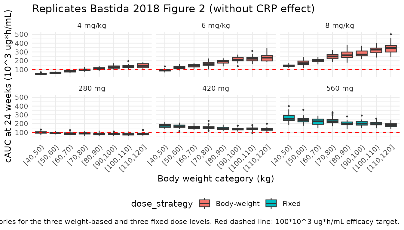
PKNCA validation
Non-compartmental analysis of the final (steady-state) Q28d dosing interval gives Cmax and Cmin for each subject and arm. The per-subject results are then summarised as mean (SD), the same format reported in Bastida 2018 Table 3.
ss_start <- tau_h * (n_doses - 1)
ss_end   <- ss_start + tau_h

nca_conc <- sim |>
  dplyr::filter(time >= ss_start, time <= ss_end, !is.na(Cc)) |>
  dplyr::mutate(time_nom = time - ss_start) |>
  dplyr::select(id, time = time_nom, Cc, treatment)

# One dose per subject per arm at the start of the SS cycle.
nca_dose <- events |>
  dplyr::filter(evid == 1, time == ss_start) |>
  dplyr::mutate(time = 0) |>
  dplyr::select(id, time, amt, treatment)

conc_obj <- PKNCA::PKNCAconc(nca_conc, Cc ~ time | treatment + id)
dose_obj <- PKNCA::PKNCAdose(nca_dose, amt ~ time | treatment + id)

intervals <- data.frame(
  start   = 0,
  end     = tau_h,
  cmax    = TRUE,
  cmin    = TRUE,
  tmax    = TRUE,
  auclast = TRUE
)

nca_res <- PKNCA::pk.nca(PKNCA::PKNCAdata(conc_obj, dose_obj, intervals = intervals))
summary(nca_res)
#>  start end treatment   N      auclast        cmax        cmin              tmax
#>      0 672    280 mg 200 14600 [16.6] 60.8 [26.9] 0.968 [568] 1.00 [1.00, 1.00]
#>      0 672   4 mg/kg 200 16800 [38.0] 67.9 [40.6]  1.51 [439] 1.00 [1.00, 1.00]
#>      0 672    420 mg 200 25500 [17.3] 95.7 [23.2]  3.74 [388] 1.00 [1.00, 1.00]
#>      0 672    560 mg 200 36900 [20.1]  134 [22.3]  7.55 [255] 1.00 [1.00, 1.00]
#>      0 672   6 mg/kg 200 29000 [33.9]  110 [38.7]  4.40 [287] 1.00 [1.00, 1.00]
#>      0 672   8 mg/kg 200 42000 [31.3]  145 [37.1]  11.7 [148] 1.00 [1.00, 1.00]
#>
#> Caption: auclast, cmax, cmin: geometric mean and geometric coefficient of variation; tmax: median and range; N: number of subjects
Comparison against Bastida 2018 Table 3 (without CRP effect)
Bastida 2018 Table 3 (p721) reports simulated steady-state mean (SD) cAUC, Cmax, and Cmin at 24 weeks of treatment under both dosing strategies, with CRP set to the reference (i.e. no CRP effect on CL). The simulated values below come directly from this vignette’s 6-cycle (24-week) simulation.
sim_summary <- cauc_per_subj |>
  dplyr::group_by(treatment) |>
  dplyr::summarise(
    cAUC_sim_mean = mean(cAUC, na.rm = TRUE) / 1e3,
    cAUC_sim_sd   = sd(cAUC,   na.rm = TRUE) / 1e3,
    Cmax_sim_mean = mean(Cmax, na.rm = TRUE),
    Cmax_sim_sd   = sd(Cmax,   na.rm = TRUE),
    Cmin_sim_mean = mean(Cmin, na.rm = TRUE),
    Cmin_sim_sd   = sd(Cmin,   na.rm = TRUE),
    .groups = "drop"
  )

published <- tibble::tibble(
  treatment     = c("4 mg/kg", "6 mg/kg", "8 mg/kg",
                    "280 mg",  "420 mg",  "560 mg"),
  cAUC_pub_mean = c(103.9, 176.9, 253.8,  87.8, 151.9, 220.2),
  cAUC_pub_sd   = c( 35.3,  56.9,  78.2,  14.3,  26.4,  39.7),
  Cmax_pub_mean = c( 72.9, 113.6, 155.6,  63.2,  98.6, 135.5),
  Cmax_pub_sd   = c( 28.4,  42.4,  56.3,  17.5,  25.0,  32.6),
  Cmin_pub_mean = c(  3.4,   9.3,  16.6,   2.4,   7.3,  13.9),
  Cmin_pub_sd   = c(  3.8,   8.1,  12.3,   2.5,   6.2,  10.1)
) |>
  dplyr::mutate(treatment = factor(treatment,
                                   levels = c("4 mg/kg", "6 mg/kg", "8 mg/kg",
                                              "280 mg",  "420 mg",  "560 mg")))

comparison <- sim_summary |>
  dplyr::left_join(published, by = "treatment") |>
  dplyr::mutate(
    cAUC_pct_diff = 100 * (cAUC_sim_mean - cAUC_pub_mean) / cAUC_pub_mean,
    Cmax_pct_diff = 100 * (Cmax_sim_mean - Cmax_pub_mean) / Cmax_pub_mean,
    Cmin_pct_diff = 100 * (Cmin_sim_mean - Cmin_pub_mean) / Cmin_pub_mean
  ) |>
  dplyr::select(treatment,
                cAUC_pub_mean, cAUC_sim_mean, cAUC_pct_diff,
                Cmax_pub_mean, Cmax_sim_mean, Cmax_pct_diff,
                Cmin_pub_mean, Cmin_sim_mean, Cmin_pct_diff) |>
  dplyr::arrange(treatment)

knitr::kable(comparison, digits = 1,
  caption = paste("Simulated vs. Bastida 2018 Table 3 mean steady-state",
                  "cAUC at 24 weeks (10^3 ug*h/mL), Cmax (ug/mL), and",
"Cmin (ug/mL) without considering the CRP effect."))| treatment | cAUC_pub_mean | cAUC_sim_mean | cAUC_pct_diff | Cmax_pub_mean | Cmax_sim_mean | Cmax_pct_diff | Cmin_pub_mean | Cmin_sim_mean | Cmin_pct_diff |
|---|---|---|---|---|---|---|---|---|---|
| 4 mg/kg | 103.9 | 105.5 | 1.5 | 72.9 | 72.9 | 0.0 | 3.4 | 3.7 | 8.1 |
| 6 mg/kg | 176.9 | 178.9 | 1.1 | 113.6 | 117.8 | 3.7 | 9.3 | 8.5 | -8.5 |
| 8 mg/kg | 253.8 | 255.1 | 0.5 | 155.6 | 154.5 | -0.7 | 16.6 | 16.8 | 1.3 |
| 280 mg | 87.8 | 87.6 | -0.3 | 63.2 | 63.0 | -0.3 | 2.4 | 2.3 | -5.6 |
| 420 mg | 151.9 | 151.4 | -0.3 | 98.6 | 98.3 | -0.3 | 7.3 | 7.4 | 0.7 |
| 560 mg | 220.2 | 218.9 | -0.6 | 135.5 | 136.8 | 1.0 | 13.9 | 13.1 | -5.4 |
Assumptions and deviations
-
Virtual-cohort weight distribution. The vignette
uses 200 subjects per dose arm with
WT ~ Uniform(40, 120), matching the Bastida 2018 Monte Carlo simulation design (p718) but with smallern(the paper used n = 1000 per arm) to keep the vignette under the 5-minute pkgdown render budget. Per-arm percentages of subjects reaching the cAUC = 100 x 10^3 ug*h/mL efficacy target are therefore noisier than the paper’s values by a factor ofsqrt(1000/200) ~ 2.2. -
CRP held at the reference (0.484 mg/dL). The
primary comparison reproduces Bastida 2018 Table 3 (“without considering
the influence of CRP”). The Table 4 scenario (CRP = 2.8 mg/dL) is not
reproduced in this vignette to keep the validation focused; users can
rebuild the events table with
crp = 2.8to obtain it. The linear additive-offset form(1 + 0.131 * (CRP - 0.484))means that holding CRP at 0.484 mg/dL zeros out the CRP effect exactly. - CRP supplied as a per-subject covariate, not time-varying. The paper assesses CRP as a time-varying covariate (Methods, p717) but the paper’s own Monte Carlo simulations use a single fixed CRP value per scenario (Tables 3 and 4). The vignette follows the paper’s simulation convention; downstream users with time-varying CRP data should supply CRP at every observation row in the event table.
- No subject-level observed data. Bastida 2018 does not release subject-level concentrations; the validation reproduces Table 3 summary statistics and Figure 2’s per-weight-category cAUC distributions rather than overlaying observed points.
- Simulation horizon. Six Q28d doses (24 weeks = 168 days = 4032 h) match the Bastida 2018 cAUC integration window exactly.
-
Dosing implementation. Doses are administered as
1-hour IV infusions with
dur = 1(model time unit = hour). Tocilizumab has a flat dosing schedule of 4, 6, or 8 mg/kg every 28 days (Bastida 2018 Methods, p717).