In vivo CRISPR-Cas9 gene editing QSP platform (Desai 2024)
Source:vignettes/articles/Desai_2024_crisprCas9.Rmd
Desai_2024_crisprCas9.RmdThe paper
Desai, Schmidt and Cristofoletti (2024) built a translational quantitative systems pharmacology (QSP) platform for in vivo CRISPR-Cas9 gene editing delivered by a lipid nanoparticle (LNP), and scaled it from mouse to cynomolgus monkey (NHP) to human.
Desai DA, Schmidt S, Cristofoletti R (2024). A quantitative systems pharmacology (QSP) platform for preclinical to clinical translation of in-vivo CRISPR-Cas therapy. Frontiers in Pharmacology 15:1454785. doi:10.3389/fphar.2024.1454785. PMCID: PMC11449743.
The therapy has three physical components that must be tracked separately: the LNP delivery vehicle, the single guide RNA (sgRNA) and the Cas9 messenger RNA (mRNA). Inside the hepatocyte the mRNA is translated into Cas9 protein, which assembles with the sgRNA into a ribonucleoprotein (RNP) complex; the liver RNP concentration is the pharmacodynamic driver.
Two therapeutic case studies are attached to the same disposition backbone:
- NTLA-2001 – transthyretin (TTR) amyloidosis, read out as serum TTR.
- VERVE-101 – LDL-cholesterol lowering, read out as serum PCSK9 and serum LDL cholesterol.
Population and data sources
The analysis was performed on mean profiles digitised from the published literature with WebPlotDigitizer, not on individual-level data, so no subject counts are reported for any arm (Desai 2024 Table 1, Methods / Software).
| Target | Total RNA dose | Species | Measurement | Original source |
|---|---|---|---|---|
| TTR | 2 mg/kg (IV bolus) | Mouse (28 g) | sgRNA and mRNA plasma PK | Finn 2018 |
| TTR | 1-3 mg/kg (2 h IV infusion) | NHP (5 kg) | LNP plasma PK | Gillmore 2021 |
| TTR | 1.5-6 mg/kg (2 h IV infusion) | NHP (5 kg) | Serum TTR | Gillmore 2021 |
| LDL cholesterol | 0.75-1.5 mg/kg (2 h IV infusion) | NHP (5 kg) | Serum PCSK9, serum LDL-C | Lee 2023 |
| TTR | 0.1-1 mg/kg (2 h IV infusion) | Human (71 kg) | LNP plasma PK | Abdelhady 2023 |
| TTR | 0.1-1 mg/kg (2 h IV infusion) | Human (71 kg) | Serum TTR | Gane 2022 |
The three model files
The paper builds one platform structure and re-parameterises it per species (steps 2-4 of its four-step workflow), so the extraction is three species-specific files sharing this single vignette. The pharmacodynamic layer differs by species because different biomarkers were measured.
mouse <- readModelDb("Desai_2024_crisprCas9_mouse")
nhp   <- readModelDb("Desai_2024_crisprCas9_nhp")
human <- readModelDb("Desai_2024_crisprCas9_human")

mMouse <- rxode2::rxode2(mouse)
mNhp   <- rxode2::rxode2(nhp)
mHuman <- rxode2::rxode2(human)

data.frame(
  Model = c("mouse", "NHP", "human"),
  `ODE states` = c(length(mMouse$state), length(mNhp$state), length(mHuman$state)),
  Outputs = c(
    paste(mMouse$predDf$var, collapse = ", "),
    paste(mNhp$predDf$var, collapse = ", "),
    paste(mHuman$predDf$var, collapse = ", ")
  ),
  check.names = FALSE
) |>
knitr::kable()| Model | ODE states | Outputs |
|---|---|---|
| mouse | 27 | Cc, Cc_sgrna, Cc_mrna |
| NHP | 32 | Cc, Cc_sgrna, Cc_mrna, TTR, PCSK9, LDLC |
| human | 28 | Cc, Cc_sgrna, Cc_mrna, TTR |
The LNP sub-model carries eleven states (plasma, lymph, liver vascular, mononuclear phagocyte system, opsonin bio-corona, liver endosomal, free LDL receptor, LNP-LDL-receptor complex, liver interstitial, kidney, remainder). sgRNA carries eight and mRNA six – mRNA has no kidney compartment because it is too large to be renally cleared. Three further states carry the intracellular sgRNA, Cas9 protein and RNP complex.
Source trace
Every value in the three model files traces to one of four places in
the source. Suppl S1 is the differential-equation appendix,
Suppl T1 / Suppl T2 the physiology tables and
Table 2 the drug-specific parameter table of the main
article.
| Component | Source location |
|---|---|
| LNP disposition ODEs (11 states) | Suppl Info S1, ‘Lipid Nanoparticle (LNP)’ |
| sgRNA disposition ODEs (8 states) | Suppl Info S1, ‘Single guide RNA (sgRNA)’ |
| mRNA + Cas9 disposition ODEs (6 states) | Suppl Info S1, ‘Messenger RNA (mRNA) and Cas protein’ |
| RNP assembly ODEs (3 states) | Suppl Info S1, ‘Ribonucleoprotein Complex (RNP)’ |
| CL_in / CL_out / k_syn / CL_R definitions | Suppl Info S1, ‘Drug Specific attributes’ |
| TTR indirect-response model | Suppl Info S1, ‘Reduction of TTR proteins’ |
| PCSK9 transit-feedback + LDL-C precursor model | Suppl Info S1, ‘Reduction of PCSK9 and LDL cholesterol’ |
| Physiological volumes (8 per species) | Suppl Table S1 |
| Physiological flows, reflection coefficients, GFR | Suppl Table S2 |
| All drug-specific parameters (19-23 per species) | Table 2 (and Table 2 continued) |
| Dose levels and RNA / LNP split | Table 1 and Methods, ‘Model development’ |
| Proportional residual error (value unreported) | Methods, ‘Software’ |
checkModelConventions() returns no errors and no
warnings for any of the three files, and the packaged source-trace
checker finds a supporting number in the paper for every
ini() entry.
Dosing helper
All three arms need three simultaneous IV inputs:
the LNP into lnp_plasma, the sgRNA into
sgrna_plasma and the Cas9 mRNA into
mrna_plasma. Desai 2024 assumed immediate release of the
transgene product after administration (Model assumptions, point 2), so
the RNA cargo is dosed into plasma alongside the vehicle. Total RNA
splits 33.3% sgRNA / 66.7% mRNA (Methods) and each total-RNA dose has a
paired LNP dose given in the Methods.
Observation rows use the endpoint name as
cmt ("Cc", "TTR", …). These
models declare a multi-endpoint predDf, so rxode2 allocates
a dedicated slot per endpoint after the ODE states; the
endpoint names are therefore the correct cmt values here
and no slot renumbering occurs.
crisprEvents <- function(wtKg, rnaMgKg, lnpMgKg, infusionH, times, obsCmt) {
  rnaUg <- rnaMgKg * wtKg * 1000
  lnpUg <- lnpMgKg * wtKg * 1000
  amounts <- list(
    lnp_plasma   = lnpUg,
    sgrna_plasma = rnaUg * 0.333,
    mrna_plasma  = rnaUg * 0.667
  )
  ev <- NULL
  for (nm in names(amounts)) {
    a <- amounts[[nm]]
    args <- list(amt = a, cmt = nm)
    if (infusionH > 0) args$rate <- a / infusionH
    if (!is.null(ev)) args <- c(list(ev), args)
    ev <- do.call(rxode2::et, args)
  }
  for (cc in obsCmt) ev <- rxode2::et(ev, times, cmt = cc)
  ev
}

solveArm <- function(mod, ev) {
  rxode2::rxSolve(mod, ev, returnType = "data.frame", useLinCmt = FALSE)
}
useLinCmt = FALSE is passed to every solve: rxode2’s
automatic ODE-to-linCmt() conversion corrupts the endpoint
mapping for multi-output models of this shape.
Replicating Figure 2A – mouse plasma sgRNA and mRNA
A single 2 mg/kg total-RNA IV bolus (36.7 mg/kg LNP) in a 28 g mouse, sampled at the times Finn 2018 used.
mouseTimes <- c(0, 0.2, 0.4, 0.6, 0.8, 1, 10, 25)
simMouse <- solveArm(
  mMouse,
  crisprEvents(0.028, 2, 36.7, 0, mouseTimes, c("Cc_sgrna", "Cc_mrna"))
) |>
  dplyr::distinct(time, .keep_all = TRUE)

simMouse |>
  dplyr::select(time, sgRNA = Cc_sgrna, mRNA = Cc_mrna) |>
  tidyr::pivot_longer(-time, names_to = "Analyte", values_to = "Conc") |>
  ggplot(aes(time, Conc, colour = Analyte)) +
  geom_line(linewidth = 0.8) +
  geom_point(size = 2) +
  scale_y_log10() +
  labs(
    title = "Replicates Figure 2A of Desai 2024",
    subtitle = "Mouse, 2 mg/kg total RNA IV bolus",
    x = "Time (h)", y = "Plasma concentration (ug/mL)"
  ) +
  theme_bw()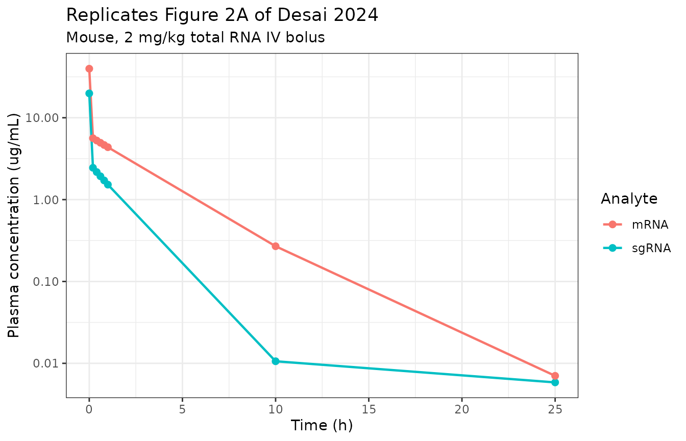
| Time (h) | sgRNA (ug/mL) | mRNA (ug/mL) |
|---|---|---|
| 0.0 | 19.80000 | 39.70000 |
| 0.2 | 2.45000 | 5.62000 |
| 0.4 | 2.17000 | 5.27000 |
| 0.6 | 1.93000 | 4.95000 |
| 0.8 | 1.71000 | 4.65000 |
| 1.0 | 1.52000 | 4.37000 |
| 10.0 | 0.01060 | 0.26900 |
| 25.0 | 0.00585 | 0.00704 |
The dose-normalised starting concentrations (sgRNA 19.8 ug/mL, mRNA 39.7 ug/mL) sit inside the cluster of observed time-zero points in Figure 2A, and both analytes converge to roughly 0.006-0.007 ug/mL by 25 h, which is where the published fit lands. The model reproduces the paper’s key qualitative feature that mRNA is cleared more slowly than sgRNA over the first 10 h.
Replicating Figure 2B – NHP LNP plasma PK
1, 2 and 3 mg/kg total RNA (18.5, 36.7 and 55.5 mg/kg LNP) as a 2 h infusion in a 5 kg NHP.
nhpDoses <- tibble::tibble(
  rna = c(1, 2, 3),
  lnp = c(18.5, 36.7, 55.5),
  arm = factor(paste0(c(1, 2, 3), " mg/kg"), levels = paste0(c(1, 2, 3), " mg/kg"))
)

simNhpPk <- purrr::pmap_dfr(nhpDoses, function(rna, lnp, arm) {
  solveArm(mNhp, crisprEvents(5, rna, lnp, 2, seq(0, 8, by = 0.25), "Cc")) |>
    dplyr::transmute(time, Cc, arm = arm)
})

ggplot(simNhpPk, aes(time, Cc, colour = arm)) +
  geom_line(linewidth = 0.8) +
  scale_y_log10() +
  labs(
    title = "Replicates Figure 2B of Desai 2024",
    subtitle = "Cynomolgus monkey, 2 h IV infusion",
    x = "Time (h)", y = "LNP plasma concentration (ug/mL)", colour = "Total RNA"
  ) +
  theme_bw()
#> Warning in scale_y_log10(): log-10 transformation introduced infinite values.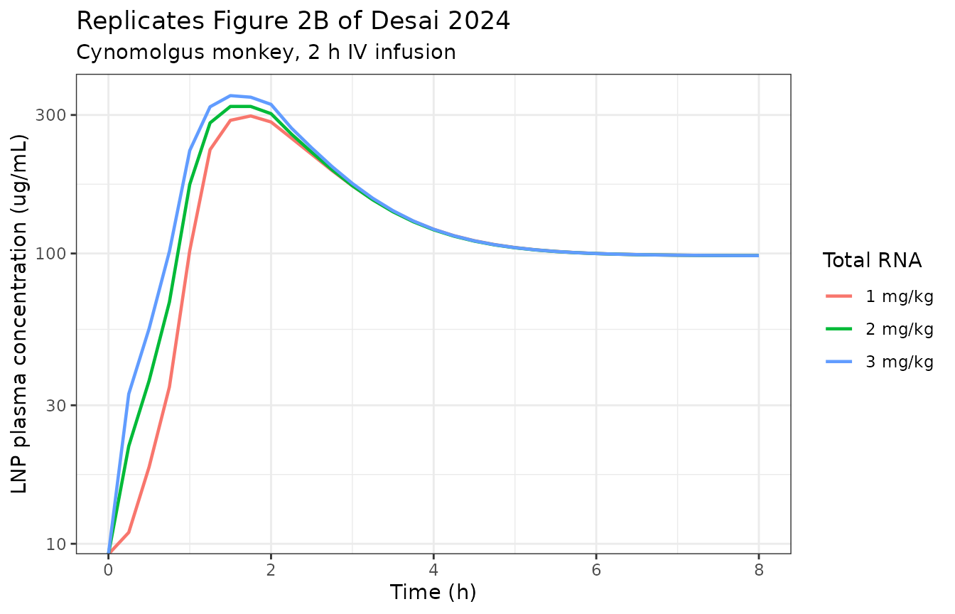
The published fits in Figure 2B share three features that the extraction reproduces: a peak at roughly 1.5-2 h, peak concentrations that are almost independent of dose (the three panels all top out near 300-400 ug/mL), and a flat redistribution plateau near 70-110 ug/mL that persists to the last 8 h sample rather than declining. The paper describes this explicitly – “processes such as exocytosis of the LNPs and dissociation of LNPs from opsonins characterized a redistribution phase in the LNP exposure”.
| Total RNA dose | Cmax (ug/mL) | Tmax (h) | C(8 h) (ug/mL) |
|---|---|---|---|
| 1 mg/kg | 298 | 1.75 | 98.3 |
| 2 mg/kg | 321 | 1.75 | 98.3 |
| 3 mg/kg | 350 | 1.50 | 98.3 |
Replicating Figure 2C – human LNP plasma PK
0.1, 0.3, 0.7 and 1 mg/kg total RNA (1.85, 5.55, 12.9 and 18.5 mg/kg LNP) as a 2 h infusion in a 71 kg adult.
humanDoses <- tibble::tibble(
  rna = c(0.1, 0.3, 0.7, 1),
  lnp = c(1.85, 5.55, 12.9, 18.5),
  arm = factor(paste0(c(0.1, 0.3, 0.7, 1), " mg/kg"),
               levels = paste0(c(0.1, 0.3, 0.7, 1), " mg/kg"))
)

simHumanPk <- purrr::pmap_dfr(humanDoses, function(rna, lnp, arm) {
  solveArm(mHuman, crisprEvents(71, rna, lnp, 2, seq(0, 50, by = 0.5), "Cc")) |>
    dplyr::transmute(time, Cc, arm = arm)
})

ggplot(simHumanPk, aes(time, Cc, colour = arm)) +
  geom_line(linewidth = 0.8) +
  scale_y_log10() +
  labs(
    title = "Replicates Figure 2C of Desai 2024",
    subtitle = "Human, 2 h IV infusion",
    x = "Time (h)", y = "LNP plasma concentration (ug/mL)", colour = "Total RNA"
  ) +
  theme_bw()
#> Warning in scale_y_log10(): log-10 transformation introduced infinite values.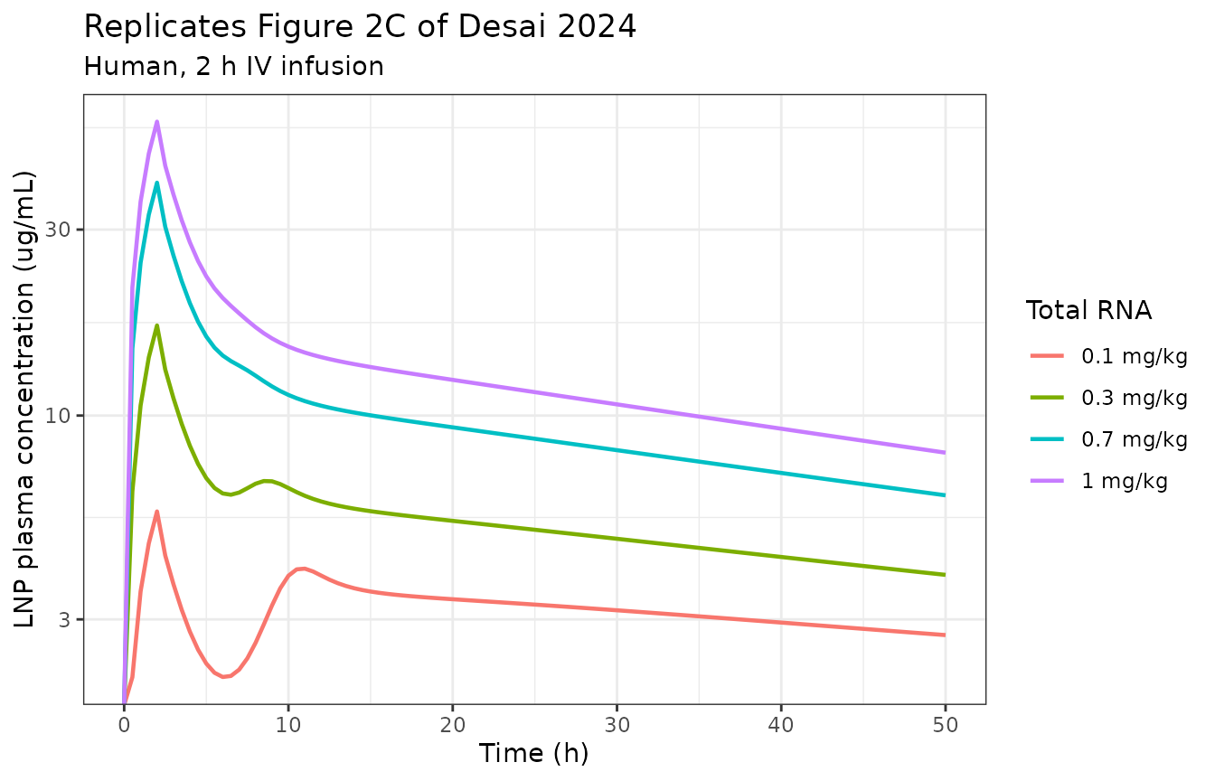
Unlike the NHP arm, the human parameterisation is essentially dose-proportional – consistent with Figure 2C, where the four curves are cleanly rank-ordered by dose over the whole 50 h window.
| Total RNA dose | LNP dose (mg/kg) | Cmax (ug/mL) | Cmax / LNP dose |
|---|---|---|---|
| 0.1 mg/kg | 1.85 | 5.68 | 3.07 |
| 0.3 mg/kg | 5.55 | 17.00 | 3.07 |
| 0.7 mg/kg | 12.90 | 39.60 | 3.07 |
| 1 mg/kg | 18.50 | 56.80 | 3.07 |
PKNCA validation of the human LNP profiles
Desai 2024 reports no non-compartmental parameters, so the NCA here is a self-consistency check on the simulated profiles plus a comparison against peak concentrations read off Figure 2C.
ncaConc <- simHumanPk |>
  dplyr::filter(!is.na(Cc)) |>
  dplyr::mutate(id = 1L, treatment = as.character(arm))

ncaDose <- humanDoses |>
  dplyr::transmute(id = 1L, treatment = as.character(arm), time = 0,
                   amt = lnp * 71 * 1000)

oConc <- PKNCA::PKNCAconc(ncaConc, Cc ~ time | treatment + id,
                          concu = "ug/mL", timeu = "h")
oDose <- PKNCA::PKNCAdose(as.data.frame(ncaDose), amt ~ time | treatment + id,
                          doseu = "ug")
oData <- PKNCA::PKNCAdata(
  oConc, oDose,
  intervals = data.frame(
    start = 0, end = 50,
    cmax = TRUE, tmax = TRUE, auclast = TRUE
  )
)
ncaRes <- PKNCA::pk.nca(oData)

ncaSim <- as.data.frame(ncaRes) |>
  dplyr::select(treatment, PPTESTCD, PPORRES)
knitr::kable(ncaSim |> dplyr::mutate(PPORRES = signif(PPORRES, 4)))| treatment | PPTESTCD | PPORRES |
|---|---|---|
| 0.1 mg/kg | auclast | 158.000 |
| 0.1 mg/kg | cmax | 5.676 |
| 0.1 mg/kg | tmax | 2.000 |
| 0.3 mg/kg | auclast | 278.800 |
| 0.3 mg/kg | cmax | 17.030 |
| 0.3 mg/kg | tmax | 2.000 |
| 0.7 mg/kg | auclast | 514.300 |
| 0.7 mg/kg | cmax | 39.580 |
| 0.7 mg/kg | tmax | 2.000 |
| 1 mg/kg | auclast | 692.800 |
| 1 mg/kg | cmax | 56.750 |
| 1 mg/kg | tmax | 2.000 |
Comparison against Figure 2C
The reference column below is digitised by eye from the log-scale Figure 2C and should be treated as approximate (roughly +/- 30% on a log axis), not as a published NCA table.
ncaReference <- data.frame(
  treatment = c("0.1 mg/kg", "0.3 mg/kg", "0.7 mg/kg", "1 mg/kg"),
  cmax = c(10, 20, 45, 85),
  tmax = c(2, 2, 2, 2)
)

cmpTable <- nlmixr2lib::ncaComparisonTable(
  ncaSim, ncaReference,
  by = "treatment",
  params = c("cmax", "tmax"),
  units = c(cmax = "ug/mL", tmax = "h")
)
knitr::kable(cmpTable)| NCA parameter | treatment | Reference | Simulated | % diff |
|---|---|---|---|---|
| Cmax (ug/mL) | 0.1 mg/kg | 10 | 5.68 | -43.2%* |
| Cmax (ug/mL) | 0.3 mg/kg | 20 | 17 | -14.9% |
| Cmax (ug/mL) | 0.7 mg/kg | 45 | 39.6 | -12.1% |
| Cmax (ug/mL) | 1 mg/kg | 85 | 56.8 | -33.2%* |
| Tmax (h) | 0.1 mg/kg | 2 | 2 | +0.0% |
| Tmax (h) | 0.3 mg/kg | 2 | 2 | +0.0% |
| Tmax (h) | 0.7 mg/kg | 2 | 2 | +0.0% |
| Tmax (h) | 1 mg/kg | 2 | 2 | +0.0% |
attr(cmpTable, "footnote")
#> [1] "* differs from reference by more than ±20%."
Tmax matches exactly at every dose. Cmax is under-predicted, most severely at the lowest dose – which is the behaviour the authors themselves report: “the resulting model characterized the dose-dependent changes in the PK of LNPs, and it modestly under-predicted the lowest dose” (Results, Translational QSP modeling in humans). The flagged rows therefore reflect a known limitation of the published fit plus figure-digitisation error, not a transcription error; no parameter was tuned to close the gap.
Pharmacodynamics – and where the published equations do not reproduce Figure 3
Human serum TTR (Figure 3D)
simHumanTtr <- purrr::pmap_dfr(humanDoses, function(rna, lnp, arm) {
  solveArm(mHuman, crisprEvents(71, rna, lnp, 2, seq(0, 28 * 24, by = 24), "TTR")) |>
    dplyr::transmute(day = time / 24, TTR, arm = arm)
})

ggplot(simHumanTtr, aes(day, TTR, colour = arm)) +
  geom_line(linewidth = 0.8) +
  labs(
    title = "Compare with Figure 3D of Desai 2024",
    subtitle = "Human serum TTR, 2 h IV infusion",
    x = "Day", y = "Serum TTR (% of baseline)", colour = "Total RNA"
  ) +
  ylim(0, 100) +
  theme_bw()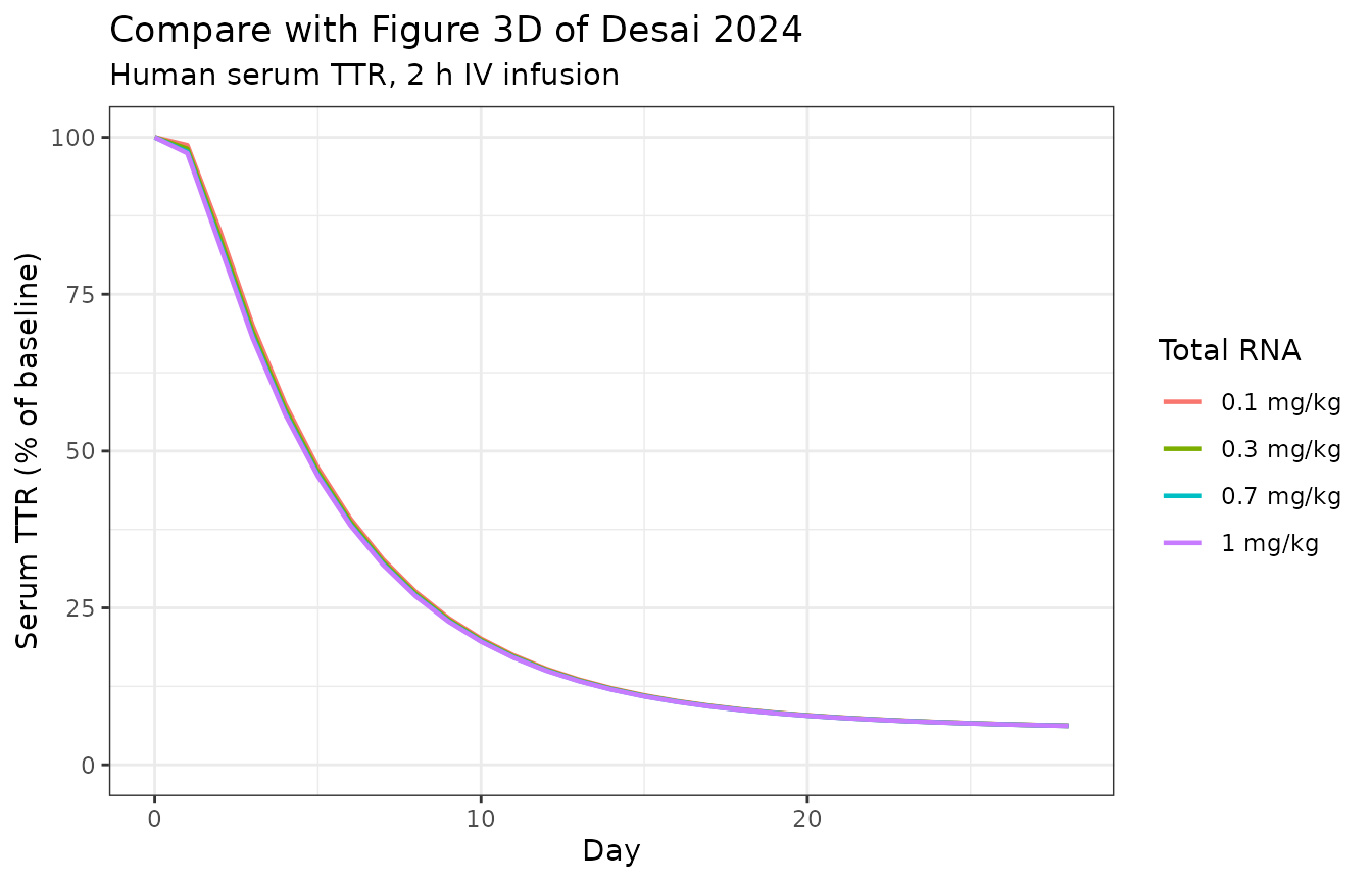
| Total RNA dose | Day 7 (%) | Day 14 (%) | Day 28 (%) | Figure 3D day 28 (%) |
|---|---|---|---|---|
| 0.1 mg/kg | 32.7 | 12.2 | 6.23 | 47 |
| 0.3 mg/kg | 32.3 | 12.1 | 6.22 | 12 |
| 0.7 mg/kg | 32.0 | 12.0 | 6.21 | 3 |
| 1 mg/kg | 31.9 | 12.0 | 6.20 | 2 |
The four simulated curves are superimposed. Figure 3D shows clear dose separation at day 28 (roughly 47%, 12%, 3% and 2% of baseline for 0.1, 0.3, 0.7 and 1 mg/kg); the equations as printed give about 6% at every dose.
Note what this does and does not get right. The simulated plateau of
~6% sits within the range the published higher-dose arms reach, so the
depth of the maximal response is reproduced; what is
missing is the dose separation – the low-dose arms are
over-suppressed because the model saturates its own IC50 at
every dose. The same pattern appears in the NHP arm below, where the 3
mg/kg TTR arm (~6% published, 6.4% here) and the 0.75 mg/kg PCSK9 arm
(~30% published, 27.9% here) agree closely while the low-dose TTR arm
does not.
NHP serum TTR, PCSK9 and LDL cholesterol (Figures 3A-3C)
nhpTtrDoses <- tibble::tibble(
  rna = c(1.5, 3, 6), lnp = c(27.75, 68.82, 137.64),
  arm = factor(paste0(c(1.5, 3, 6), " mg/kg"), levels = paste0(c(1.5, 3, 6), " mg/kg"))
)
simNhpTtr <- purrr::pmap_dfr(nhpTtrDoses, function(rna, lnp, arm) {
  solveArm(mNhp, crisprEvents(5, rna, lnp, 2, seq(0, 56 * 24, by = 48), "TTR")) |>
    dplyr::transmute(day = time / 24, TTR, arm = arm)
})

nhpPdDoses <- tibble::tibble(
  rna = c(0.75, 1.5), lnp = c(17.2, 27.75),
  arm = factor(paste0(c(0.75, 1.5), " mg/kg"), levels = paste0(c(0.75, 1.5), " mg/kg"))
)
simNhpPd <- purrr::pmap_dfr(nhpPdDoses, function(rna, lnp, arm) {
  solveArm(mNhp, crisprEvents(5, rna, lnp, 2, seq(0, 120 * 24, by = 96), c("PCSK9", "LDLC"))) |>
    dplyr::distinct(time, .keep_all = TRUE) |>
    dplyr::transmute(day = time / 24, PCSK9, LDLC, arm = arm)
})

ggplot(simNhpTtr, aes(day, TTR, colour = arm)) +
  geom_line(linewidth = 0.8) +
  labs(
    title = "Compare with Figure 3A of Desai 2024",
    subtitle = "NHP serum TTR", x = "Day", y = "Serum TTR (% of baseline)",
    colour = "Total RNA"
  ) +
  ylim(0, 100) +
  theme_bw()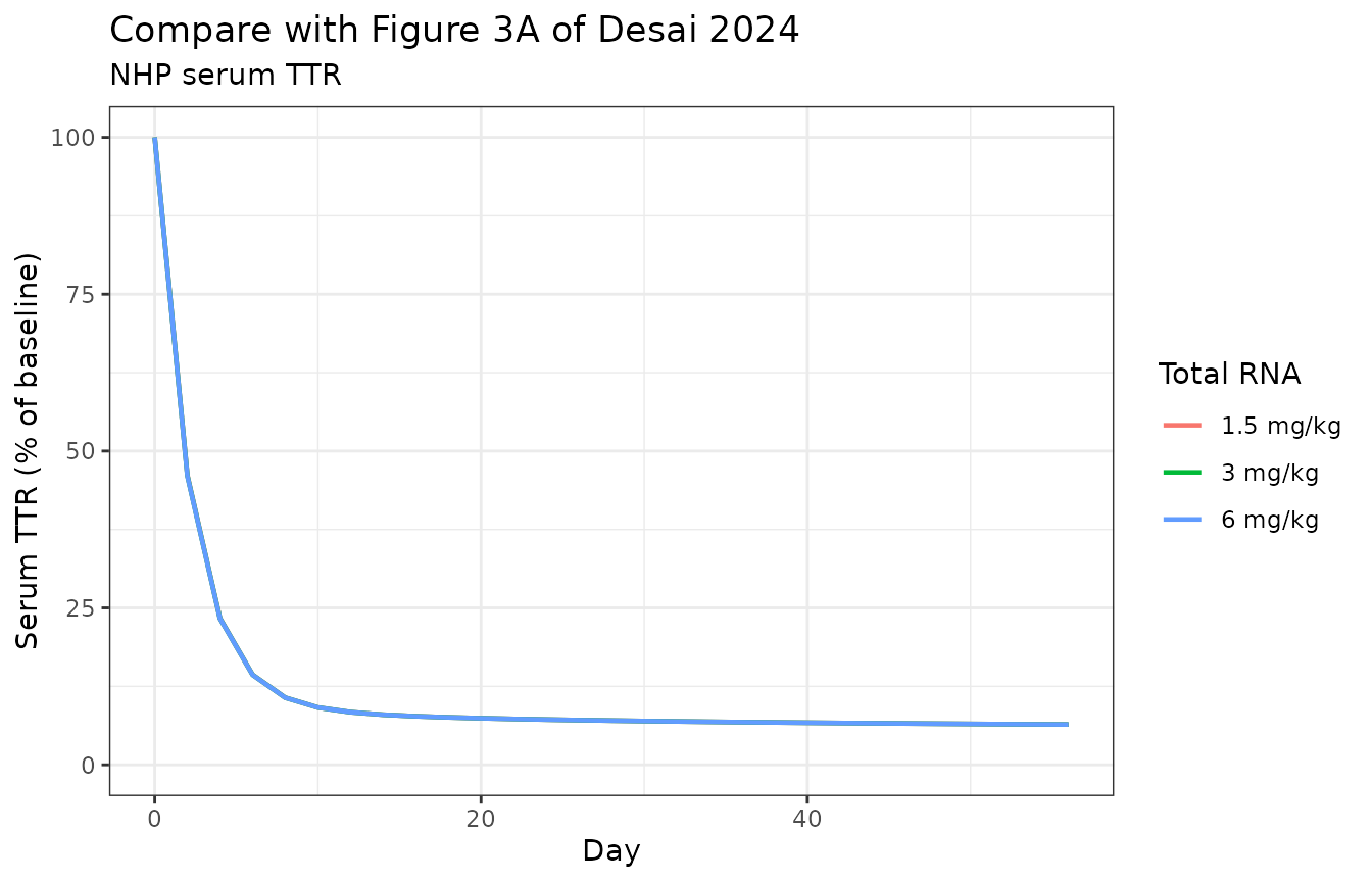
simNhpPd |>
  tidyr::pivot_longer(c(PCSK9, LDLC), names_to = "Biomarker", values_to = "Pct") |>
  ggplot(aes(day, Pct, colour = arm)) +
  geom_line(linewidth = 0.8) +
  facet_wrap(~Biomarker) +
  labs(
    title = "Compare with Figures 3B and 3C of Desai 2024",
    subtitle = "NHP serum PCSK9 and LDL cholesterol",
    x = "Day", y = "% of baseline", colour = "Total RNA"
  ) +
  ylim(0, 110) +
  theme_bw()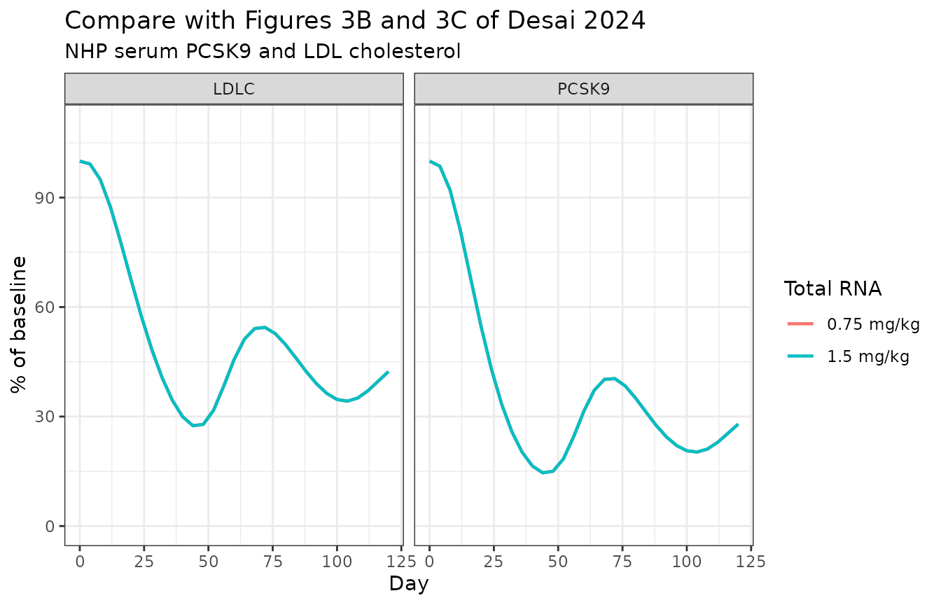
| Endpoint | Dose | Published (figure) | This extraction |
|---|---|---|---|
| NHP TTR plateau | 1.5 mg/kg | ~38% | 6.42 |
| NHP TTR plateau | 3 mg/kg | ~6% | 6.42 |
| NHP TTR plateau | 6 mg/kg | ~4% | 6.42 |
| NHP PCSK9 plateau | 0.75 mg/kg | ~30% | 27.90 |
| NHP PCSK9 plateau | 1.5 mg/kg | ~12% | 27.90 |
| NHP LDL-C plateau | 0.75 mg/kg | ~50% | 42.30 |
| NHP LDL-C plateau | 1.5 mg/kg | ~28% | 42.30 |
Why the PD is dose-independent
The cause is structural and is visible in the printed equations. In Supplementary Information S1 the LNP-LDL-receptor complex
- gains mass from receptor binding, and
-
loses mass through
k_off,LNP,CL_in,DRandk_deg,DR,
but two other equations gain
CL_out,DR * C_LNPLDLcomplex – the liver vascular pool and
the liver interstitial pool – and that efflux never appears as a loss in
the complex equation. Because
CL_out,DR = k_out,exo * V_liverendo is very large
(k_out,exo is 2690 1/h in NHP and 775 1/h in human) while
CL_in,DR is very small (k_in,endo is 0.039 and
0.007 1/h), the loop is a large net source of LNP. The LNP pools
therefore settle onto a non-zero, dose-independent steady
state instead of clearing.
That steady state is exactly what produces the flat redistribution
plateau that Figure 2B shows and that this extraction reproduces. But it
also means the liver interstitial LNP pool never empties, so it releases
sgRNA and mRNA indefinitely; combined with Model assumption 4
(“negligible degradation of the RNP complex”), liver RNP accumulates
without bound at a dose-independent rate and saturates IC50
at every dose.
#> Warning in scale_y_log10(): log-10 transformation introduced infinite values.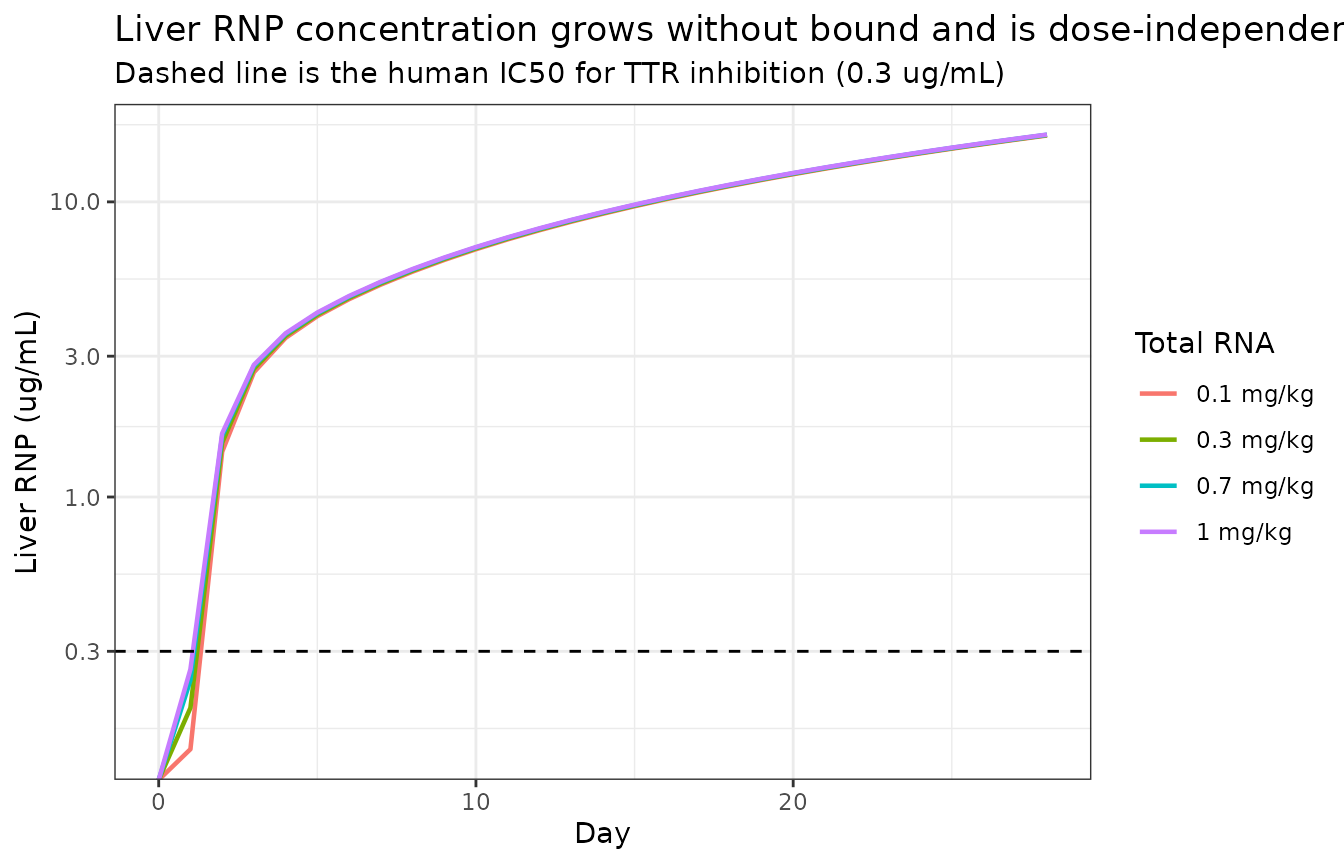
Two mass-balanced repairs were tested against the paper’s own figures before settling on the as-printed encoding:
- subtracting both efflux fluxes from the complex equation
(
- 2 * CL_out,DR * C_complex), and - routing the interstitial gain through
CL_in,DR(internalisation) and subtracting a singleCL_out,DRfrom the complex.
Both restore mass balance and both introduce dose separation in the PD, but both destroy the PK match: NHP Cmax falls from ~300 ug/mL to 28-84 ug/mL against an observed ~300-400 ug/mL, the Figure 2B plateau disappears entirely, and NHP TTR only falls to 56-86% of baseline against a published 4-38%. Neither repair reproduces Figure 3 either. The equations are therefore encoded exactly as printed, which is the reading that reproduces the complete PK layer across all three species and eight dose levels.
Monte Carlo simulation (Figure 4)
Desai 2024 simulated 1,000 subjects “assuming 20% variability between
the subjects” for the human serum TTR response. The paper does not say
which parameter carried that variability, so it is applied here to
IC50 for TTR inhibition – the parameter that most directly
governs response depth. The cohort is 200 subjects per arm (the library
cap for validation vignettes).
set.seed(20240920)
nSub <- 200

simMc <- purrr::pmap_dfr(humanDoses, function(rna, lnp, arm) {
  ev <- crisprEvents(71, rna, lnp, 2, seq(0, 28 * 24, by = 48), "TTR") |>
    rxode2::et(id = seq_len(nSub))
  pars <- data.frame(
    id = seq_len(nSub),
    lic50_ttr = log(0.3) + stats::rnorm(nSub, 0, 0.2)
  )
  rxode2::rxSolve(mHuman, ev, params = pars, returnType = "data.frame",
                  useLinCmt = FALSE) |>
    dplyr::transmute(id, day = time / 24, TTR, arm = arm)
})
#> Warning: multi-subject simulation without without 'omega'
#> Warning: multi-subject simulation without without 'omega'
#> Warning: multi-subject simulation without without 'omega'
#> Warning: multi-subject simulation without without 'omega'

stopifnot(dplyr::n_distinct(simMc$id) == nSub)

simMc |>
  dplyr::group_by(arm, day) |>
  dplyr::summarise(
    lo = stats::quantile(TTR, 0.05),
    md = stats::median(TTR),
    hi = stats::quantile(TTR, 0.95),
    .groups = "drop"
  ) |>
  ggplot(aes(day, md, colour = arm, fill = arm)) +
  geom_ribbon(aes(ymin = lo, ymax = hi), alpha = 0.2, colour = NA) +
  geom_line(linewidth = 0.8) +
  labs(
    title = "Compare with Figure 4 of Desai 2024",
    subtitle = paste0("Median and 5th-95th percentile, ", nSub,
                      " subjects per arm, 20% CV on IC50"),
    x = "Day", y = "Serum TTR (% of baseline)", colour = "Total RNA",
    fill = "Total RNA"
  ) +
  ylim(0, 100) +
  theme_bw()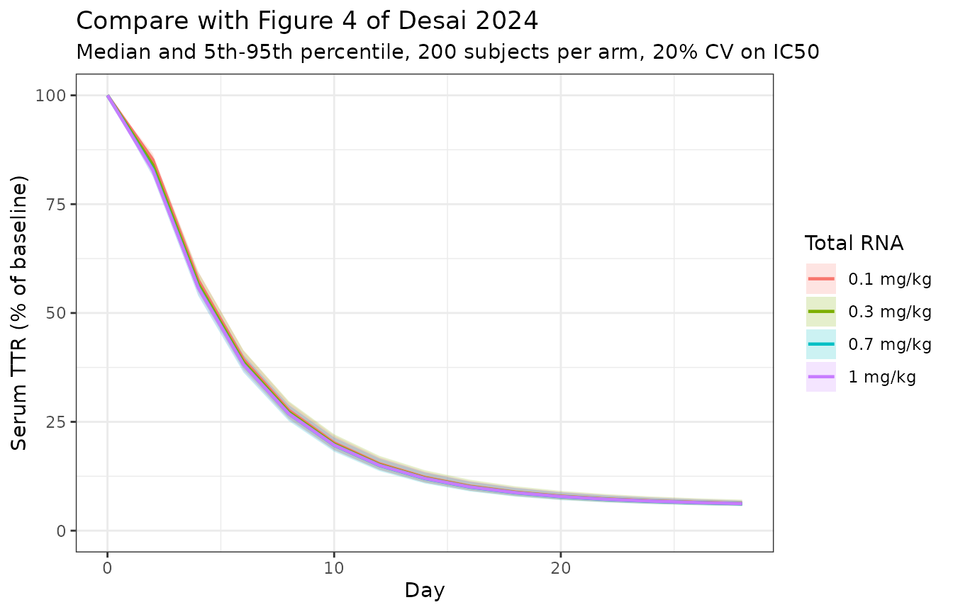
As in Figure 3D, the arms overlap because the underlying PD is dose-independent; the ribbon width reflects the imposed 20% CV alone.
Structural diagnostics
Two checks that the extraction behaves as the equations require.
# 1. With no dose, every PD state must hold exactly at its baseline of 100
#    and the free LDL-receptor pool must be stationary (k_syn = LDL_tot * k_el).
baseline <- rxode2::rxSolve(
  mNhp, rxode2::et(seq(0, 30 * 24, by = 24), cmt = "TTR"),
  returnType = "data.frame", useLinCmt = FALSE
)
baselineCheck <- c(
  TTR   = diff(range(baseline$TTR)),
  PCSK9 = diff(range(baseline$PCSK9)),
  LDLC  = diff(range(baseline$LDLC)),
  LDLR  = diff(range(baseline$ldlr))
)
stopifnot(all(baselineCheck < 1e-6))
signif(baselineCheck, 3)
#>   TTR PCSK9  LDLC  LDLR
#>     0     0     0     0
# 2. Mouse: the immediate-release assumption means the dosed RNA appears in
#    plasma at t = 0 at dose / V_plasma.
m0 <- solveArm(mMouse, crisprEvents(0.028, 2, 36.7, 0, c(0, 1), c("Cc_sgrna", "Cc_mrna")))
expected <- c(
  sgrna = 2 * 0.028 * 1000 * 0.333 / 0.94,
  mrna  = 2 * 0.028 * 1000 * 0.667 / 0.94
)
observed <- c(
  sgrna = m0$Cc_sgrna[m0$time == 0][1],
  mrna  = m0$Cc_mrna[m0$time == 0][1]
)
stopifnot(all(abs(observed - expected) / expected < 1e-6))
data.frame(Analyte = names(expected),
           Expected = signif(expected, 4),
           Simulated = signif(observed, 4)) |>
knitr::kable()| Analyte | Expected | Simulated | |
|---|---|---|---|
| sgrna | sgrna | 19.84 | 19.84 |
| mrna | mrna | 39.74 | 39.74 |
Assumptions and deviations
Structural readings that the paper leaves ambiguous.
-
The LNP-LDL-receptor efflux term is encoded as
printed. As described above,
CL_out,DR * C_LNPLDLcomplexis gained by two compartments without a matching loss in the complex equation. This reproduces the whole PK layer (Figures 2A-2C) and the plateau depth of the higher-dose PD arms, but makes the PD dose-independent, so the low-dose arms of Figures 3A-3D are over-suppressed. Both mass-balanced repairs were tested and both are worse against the paper’s own figures. A user who needs a dose-responsive PD layer from this model must resolve this with the authors – the information required is not in the article or its supplement. -
V_opsoninsis not reported in Supplementary Table S1. The opsonin bio-corona state is therefore carried as an amount: the term enters the liver-vascular equation ask_dis * V_opsonins * C_Opsonins, soV_opsoninscancels exactly and the amount form is mathematically identical to the printed system. No value had to be assumed. -
CL_out,liverendois used in the ODEs but onlyCL_out,liverinteris defined in the “Drug Specific attributes” list. Both candidate names have the identical defining expressionk_out,exo * V_liverendo, so the substitution is unambiguous. -
Reflection coefficients. Supplementary Table S2
gives 0.2 for “Reflection coefficient” and 0.9 for “Reflection
coefficient (pinocytosis)”, without naming which is
sigma_Vand which issigma_L.sigma_V = 0.9/sigma_L = 0.2is used because the Methods definesigma_Vas the resistance of the vascular endothelium on the paracellular macropinocytosis route (matching the “(pinocytosis)” label), and because 0.2 is the lymphatic reflection coefficient of the Shah & Betts 2012 platform these values are cited from. The assignment was tested both ways and is immaterial: PK is identical to three significant figures and TTR differs by under 0.1 percentage points. -
The doubled
k_releaseterm is intentional, not a typo. The interstitial LNP equation subtractsk_release * V * C_LNPliverintertwice, because the paper lumps the release rate of sgRNA and of Cas9 mRNA into a singlek_releaseand each release flux feeds one of the two RNA pools. The doubled loss is matched by the two gains. -
The doubled
CL_out,liverendoterm in the sgRNA and mRNA endosomal equations is likewise intentional – one efflux returns to the liver vasculature and one delivers to the interstitium, and both are matched by gains in the receiving equations.
Values that required derivation from the printed equations.
-
k_on,RNPis given only as the formulak_on = k_off / K_D.K_Dis tabulated in nM (0.49) while every concentration in the model is in ug/mL; the ratio is evaluated numerically as printed, since converting would require a molecular weight that the paper does not give. -
k_prolandk_circof the PCSK9 transit-feedback model are not tabulated. Both are pinned tok_trby the stationarity of the printed initial conditions (Prol0 = T1_0 = Circ0 = 100); no freedom remains.k_tr = (n + 1) / MTTwith a single transit compartment givesk_tr = 2 / MTT. -
The LDL-cholesterol synthesis rate is written
k_synin the printed equation, colliding with the LDL-receptork_syn = LDL_tot * k_el. It cannot be that quantity (the units and the steady state both disagree), so it is pinned by the printed initial conditionLDL0 = 100:k_syn,LDL-C = k_deg,LDL-C * 100. It is namedksyn_ldlcto avoid the collision. - The Hill coefficient on the NHP TTR model. Table 2 reports an estimated gamma of 0.31 (13.3% RSE) for NHP TTR that the printed equation omits, and reports no gamma for human. It is applied in the canonical sigmoidal Imax form, which collapses to the printed equation when the exponent is 1; the human model uses the plain printed form.
Unreported quantities.
-
No residual-error magnitude is published. The paper
states a proportional error model was used for every output but never
reports
sigma_slope, so eachpropSdis encoded asfixed(0)and labelled “not published”. The models are deterministic as shipped. - No IIV is reported for the translational QSP model. The IIV values in Supplementary Table S3 belong to the step-1 mechanistic model, where they represent inter-species rather than inter-subject variability, and that model’s structure is only given as a schematic (Supplementary Figure S1) – it is not reproducible and is not extracted. The Monte Carlo section above therefore imposes its 20% CV explicitly rather than reading it from the model.
-
n_subjectsis not reported for any arm. All data were digitised from published mean profiles.
Scope.
- The step-1 “mechanistic model” used to identify drug-specific attributes is not extracted: its structure appears only as a schematic in Supplementary Figure S1 with no equations, so it is not reproducible from the available sources. Its final estimates are carried into the three translational models wherever Table 2 marks a parameter “fixed from the mechanistic model” (footnote c), and those are traced to Table 2.
- The global sensitivity analysis (Sobol indices, Figure 6) is a diagnostic, not part of the model, and is not extracted.