Proguanil (Khwarg 2024)
Source:vignettes/articles/Khwarg_2024_proguanil.Rmd
Khwarg_2024_proguanil.RmdModel and source
- Citation: Khwarg J, Yang E, Park CS, Ji SC, Yu K-S, Lee S. Effect of SLC22A1 polymorphism on the pharmacokinetics of proguanil in Korean: A semi-physiologic population pharmacokinetic approach. Clin Transl Sci. 2024;17:e70103. doi:10.1111/cts.70103
- Article: https://doi.org/10.1111/cts.70103
Semi-physiologic joint parent-metabolite population PK model for oral
proguanil and its active metabolite cycloguanil in healthy Korean male
adults, quantifying the effect of the SLC22A1 (OCT1) 1022C>T
(rs2282143) polymorphism on hepatic uptake (Khwarg 2024). Proguanil is
absorbed first-order from the depot directly into a
permeability- considered well-stirred liver compartment, so
hepatic first-pass metabolism is structural rather than folded into a
bioavailability term. The liver exchanges with central at
the hepatic plasma flow QH (inflow QH, return flow QH * (1 - EH)), and
central additionally exchanges with
peripheral1 at Q/F and is cleared at CL/F, the apparent
clearance via the non-cycloguanil pathway. The hepatic extraction ratio
EH follows the well-stirred model on a blood basis from the blood
unbound fraction fub, the intrinsic clearance CLint and the hepatic
blood flow QBH; the resulting hepatic plasma clearance CLH = EH * QBH *
(CB/CP) carries proguanil out of the liver and into the cycloguanil
chain. Cycloguanil is formed in liver_cycloguanil and
effluxes to central_cycloguanil through two transit
compartments with a shared rate constant mKT, then is cleared at CLM/F;
its central volume was set equal to the proguanil central volume because
the two were not separately identifiable. Liver volume (1 L) and hepatic
blood flow (90 L/h) are fixed physiologic constants for a 70 kg adult,
allometrically scaled on body weight with exponents 1 and 0.75; the
plasma unbound fraction (0.25), blood-to-plasma ratio (2.7) and
hematocrit (0.45) are fixed literature values. The SLC22A1 1022C>T
heterozygote (CT) genotype enters as an exponent on FUP = 0.416, the
relative fraction of OCT1-mediated hepatocyte uptake versus the CC wild
type, reducing EH and thereby raising proguanil and lowering cycloguanil
exposure.
This is a semi-physiologic joint parent-metabolite model: rather than attaching the transporter genotype to a systemic clearance term, Khwarg 2024 places a well-stirred liver compartment between the absorption depot and the central compartment and lets the SLC22A1 (OCT1) genotype act on the OCT1-mediated hepatocyte uptake inside the hepatic extraction ratio. That is the point of the paper – as its Discussion puts it, “directly applying a transporter genotype as a covariate to systemic clearance is not straightforward, considering that hepatic uptake and clearance do not have a proportional relationship.”
Population
The model was fit to the PK data of the CYP2C19-mediated tegoprazan/proguanil drug-drug-interaction study NCT04568772 (Khwarg 2024 Methods “Data”), using 160 proguanil and 159 cycloguanil plasma concentrations from 16 healthy Korean subjects sampled over 48 h after a single oral atovaquone/proguanil 250/100 mg dose (i.e. 100 mg proguanil hydrochloride), given alone or with tegoprazan 50 mg. The esomeprazole and vonoprazan arms of the parent study were excluded because of known interactions with proguanil.
All subjects were male, aged 19-50 y at eligibility (cohort mean 34.31 y, SD 7.38), with mean height 172.85 cm (SD 7.37), mean body weight 76.12 kg (SD 9.82) and mean BMI 25.52 kg/m^2 (SD 3.14) (Khwarg 2024 Results “Demographics”; per-genotype demographics in Table S2). Every subject was a CYP2C19 normal metabolizer (1/1), which is what isolates the SLC22A1 effect from CYP2C19 phenotype as a confounder.
Thirteen of the 16 subjects consented to genotyping. Of the six assayed decreased-function SLC22A1 SNPs, only 1022C>T (rs2282143) was polymorphic: 9 subjects were CC homozygous wild type and 4 were CT heterozygous; no TT homozygotes were observed (Khwarg 2024 Table 1). The three ungenotyped subjects were assigned by a mixture model with Hardy-Weinberg probabilities fixed at 0.7 (CC) / 0.3 (CT), and all three were classified CC.
The same information is available programmatically via the model’s
population metadata
(readModelDb("Khwarg_2024_proguanil")()$population).
Source trace
The per-parameter origin is recorded as an in-file comment next to
each ini() entry in
inst/modeldb/specificDrugs/Khwarg_2024_proguanil.R. The
table below collects them in one place for review.
| Equation / parameter | Value | Source location |
|---|---|---|
lka (KA) |
0.101 1/h | Table 3, Proguanil (RSE 6.0%) |
lcl (CL/F) |
33.5 L/h | Table 3, Proguanil (RSE 16.4%) |
lvc (Vc/F) |
58.4 L | Table 3, Proguanil (RSE 24.1%) |
lq (Q/F) |
41.4 L/h | Table 3, Proguanil (RSE 7.2%) |
lvp (Vp/F) |
1400 L | Table 3, Proguanil (RSE 26.0%) |
lclint (CLint) |
78.3 L/h | Table 3, Proguanil (RSE 18.6%) |
e_snp_oct1_clint (FUP) |
0.416 | Table 3, Proguanil (RSE 54.1%) |
lktr_cycloguanil (mKT) |
1.03 1/h | Table 3, Cycloguanil (RSE 5.8%) |
lcl_cycloguanil (CLM/F) |
97.0 L/h | Table 3, Cycloguanil (RSE 13.8%) |
etalcl |
31.7 %CV -> 0.095755 | Table 3 IIV CL/F; footnote CV = sqrt(exp(omega^2)-1)*100 |
etalvc |
87.2 %CV -> 0.565532 | Table 3 IIV Vc/F |
etalclint |
53.7 %CV -> 0.253377 | Table 3 IIV CLint |
etalktr_cycloguanil |
15.5 %CV -> 0.023741 | Table 3 IIV mKT |
propSd |
0.16 | Table 3, Proguanil proportional error (RSE 9.1%) |
propSd_cycloguanil |
0.124 | Table 3, Cycloguanil proportional error (RSE 12.7%) |
addSd_cycloguanil |
0.372 ug/L | Table 3, Cycloguanil additive error (RSE 18.5%) |
fu_fix (fu) |
0.25 | Methods “Structural model” (refs 7, 24) |
bpr_fix (CB/CP) |
2.7 | Methods “Structural model” (refs 7, 24) |
hct_fix (hematocrit) |
0.45 | Methods “Structural model” / Equation 7 |
lvh_70 (VH at 70 kg) |
1 L | Equation 5 |
lqbh_70 (QBH at 70 kg) |
90 L/h | Equation 6 |
e_wt_vh |
1 | Equation 5, (body weight / 70 kg) with no exponent |
e_wt_qbh |
0.75 | Equation 6, (body weight / 70 kg)^0.75
|
fub = fu / (CB/CP) |
n/a | Equation 3 |
eh well-stirred with FUP^GENO
|
n/a | Equation 8 (Equation 1 is its GENO = 0 case) |
CLBH = eh * QBH |
n/a | Equation 2 |
CLH = CLBH * (CB/CP) |
n/a | Equation 4 |
QH = QBH * (1 - hematocrit) |
n/a | Equation 7 |
| ODE topology (all 8 states, all flows) | n/a | Figure 2 (model schematic) |
| Molar-mass ratio 288.17 / 290.19 | 0.993004 | Results “Structural model” |
The fixed physiologic sub-model
Equations 3, 5, 6 and 7 are pure physiology and were not estimated. This chunk reproduces them independently of the model file, so the numbers the ODEs consume are visible and checkable.
wt_mean <- 76.12 # kg, Khwarg 2024 Results "Demographics"
fu <- 0.25
bpr <- 2.7
hct <- 0.45

fub <- fu / bpr # Eq 3
vh <- 1 * (wt_mean / 70)^1 # Eq 5, L
qbh <- 90 * (wt_mean / 70)^0.75 # Eq 6, L/h
qh <- qbh * (1 - hct) # Eq 7, L/h

tibble::tibble(
  Quantity = c(
    "fub = fu / (CB/CP)", "VH (L)", "QBH (L/h)", "QH (L/h)"
  ),
  Equation = c("3", "5", "6", "7"),
  Value = round(c(fub, vh, qbh, qh), 4)
) |>
knitr::kable(caption = "Fixed physiologic constants at the cohort mean body weight.")| Quantity | Equation | Value |
|---|---|---|
| fub = fu / (CB/CP) | 3 | 0.0926 |
| VH (L) | 5 | 1.0874 |
| QBH (L/h) | 6 | 95.8392 |
| QH (L/h) | 7 | 52.7115 |
The genotype effect enters Equation 8 as an exponent on FUP, then
propagates to the hepatic blood clearance (Equation 2) and the hepatic
plasma clearance (Equation 4). Because the dose is absorbed into the
liver, the fraction of an absorbed dose that survives first pass is
QH * (1 - EH) / (QH * (1 - EH) + CLH).
clint <- 78.3
fup <- 0.416

extraction <- lapply(0:1, function(geno) {
  uptake <- fub * clint * fup^geno # Eq 8 numerator term
  eh <- uptake / (qbh + uptake) # Eq 8
  cl_bh <- eh * qbh # Eq 2
  cl_h <- cl_bh * bpr # Eq 4
  back <- qh * (1 - eh) # Figure 2, liver -> central
  tibble::tibble(
    Genotype = c("CC (GENO = 0)", "CT (GENO = 1)")[geno + 1],
    EH = eh, `CLBH (L/h)` = cl_bh, `CLH (L/h)` = cl_h,
    `First-pass surviving fraction` = back / (back + cl_h)
  )
}) |>
  dplyr::bind_rows()

extraction |>
  dplyr::mutate(dplyr::across(where(is.numeric), \(x) round(x, 4))) |>
knitr::kable(caption = "Hepatic extraction by SLC22A1 1022C>T genotype (Equations 2, 4, 8).")| Genotype | EH | CLBH (L/h) | CLH (L/h) | First-pass surviving fraction |
|---|---|---|---|---|
| CC (GENO = 0) | 0.0703 | 6.7401 | 18.1983 | 0.7292 |
| CT (GENO = 1) | 0.0305 | 2.9240 | 7.8948 | 0.8662 |
The CT heterozygote’s extraction ratio is 0.434-fold that of the CC wild type – less drug is taken up into the hepatocyte, so more parent survives to systemic plasma and less cycloguanil is formed. That is exactly the mechanism the paper reports.
Virtual cohort
Original observed data are not publicly available. Two virtual arms of 200 subjects each are built, one per SLC22A1 1022C>T genotype, with body weights drawn to match the published mean and SD and truncated to the study’s BMI eligibility range at the mean height.
set.seed(20241212)

n_per_arm <- 200L
obs_times <- seq(0, 48, by = 0.5)

make_arm <- function(n, geno, label, id_offset = 0L) {
  # Body weight: mean 76.12 kg, SD 9.82 kg (Khwarg 2024 Results
  # "Demographics"), truncated to the BMI 19-30 kg/m^2 eligibility band at
  # the cohort mean height of 172.85 cm.
  ht_m <- 172.85 / 100
  wt <- pmin(pmax(rnorm(n, 76.12, 9.82), 19 * ht_m^2), 30 * ht_m^2)
  subj <- tibble::tibble(
    id = id_offset + seq_len(n),
    WT = wt,
    SNP_SLC22A1_RS2282143 = geno,
    genotype = label
  )
  dplyr::bind_rows(
    # Single oral 100 mg proguanil hydrochloride into the depot.
    subj |> dplyr::mutate(
      time = 0, amt = 100, evid = 1L,
      cmt = "depot", dvid = NA_integer_
    ),
    # Observation rows. Both model outputs are ALGEBRAIC endpoints, so the
    # observation record is addressed by `dvid` with a missing compartment;
    # rxode2 then returns every observable as a column on every output row.
    # Naming an observable in the compartment column instead would inject a
    # compartment slot for it and renumber the ODE states.
    subj |> tidyr::crossing(time = obs_times) |> dplyr::mutate(
      amt = NA_real_, evid = 0L,
      cmt = NA_character_, dvid = 1L
    )
  ) |>
    dplyr::arrange(id, time, dplyr::desc(evid))
}

events <- dplyr::bind_rows(
  make_arm(n_per_arm, 0, "CC", id_offset = 0L),
  make_arm(n_per_arm, 1, "CT", id_offset = n_per_arm)
)

stopifnot(!anyDuplicated(unique(events[, c("id", "time", "evid")])))
stopifnot(nrow(dplyr::distinct(events, id)) == 2L * n_per_arm)
Simulation
mod <- readModelDb("Khwarg_2024_proguanil")

# `useLinCmt = FALSE` -- rxode2's automatic ODE -> linCmt conversion corrupts
# the dvid -> cmt mapping for multi-output models of this shape.
sim <- rxode2::rxSolve(
  mod,
  events = events,
  keep = c("WT", "SNP_SLC22A1_RS2282143", "genotype"),
  useLinCmt = FALSE,
  returnType = "data.frame"
) |>
  dplyr::filter(!is.na(time))

# Typical-value (no between-subject variability) profiles at the cohort mean
# weight, used for the Figure 1 overlay.
typical_events <- dplyr::bind_rows(
  make_arm(1L, 0, "CC", id_offset = 0L),
  make_arm(1L, 1, "CT", id_offset = 1L)
) |>
  dplyr::mutate(WT = wt_mean)

sim_typical <- rxode2::rxSolve(
  mod,
  events = typical_events,
  keep = c("genotype"),
  omega = NA,
  useLinCmt = FALSE,
  returnType = "data.frame"
) |>
  dplyr::filter(!is.na(time))
#> Warning: multi-subject simulation without without 'omega'
Replicate published figures
Figure 1 – mean concentration-time profiles and metabolic ratio by genotype
Khwarg 2024 Figure 1 plots the mean proguanil (panel a) and cycloguanil (panel b) plasma profiles and their ratio (panel c) by genotype. The cohort means from the virtual population are overlaid with the typical-value prediction.
# Replicates Figure 1 of Khwarg 2024.
long_mean <- sim |>
  dplyr::group_by(genotype, time) |>
  dplyr::summarise(
    Proguanil = mean(Cc),
    Cycloguanil = mean(Cc_cycloguanil),
    `Cycloguanil / proguanil ratio` = mean(Cc_cycloguanil / Cc, na.rm = TRUE),
    .groups = "drop"
  ) |>
  tidyr::pivot_longer(-c(genotype, time), names_to = "panel", values_to = "value") |>
  dplyr::mutate(panel = factor(panel, levels = c(
    "Proguanil", "Cycloguanil", "Cycloguanil / proguanil ratio"
  )))

long_typ <- sim_typical |>
  dplyr::group_by(genotype, time) |>
  dplyr::summarise(
    Proguanil = mean(Cc),
    Cycloguanil = mean(Cc_cycloguanil),
    `Cycloguanil / proguanil ratio` = mean(Cc_cycloguanil / Cc, na.rm = TRUE),
    .groups = "drop"
  ) |>
  tidyr::pivot_longer(-c(genotype, time), names_to = "panel", values_to = "value") |>
  dplyr::mutate(panel = factor(panel, levels = levels(long_mean$panel)))

ggplot(long_mean, aes(time, value, colour = genotype)) +
  geom_line(linewidth = 0.9) +
  geom_line(
    data = long_typ, aes(time, value, colour = genotype),
    linetype = "dashed", linewidth = 0.5
  ) +
  facet_wrap(~panel, scales = "free_y") +
  labs(
    x = "Time (h)", y = "Plasma concentration (ug/L) or ratio",
    colour = "SLC22A1 1022C>T",
    title = "Figure 1 - mean profiles by SLC22A1 genotype",
    caption = paste(
      "Replicates Figure 1 of Khwarg 2024. Solid = virtual-cohort mean,",
      "dashed = typical value."
    )
  ) +
  theme_bw() +
  theme(legend.position = "bottom")
#> Warning: Removed 2 rows containing missing values or values outside the scale range
#> (`geom_line()`).
#> Removed 2 rows containing missing values or values outside the scale range
#> (`geom_line()`).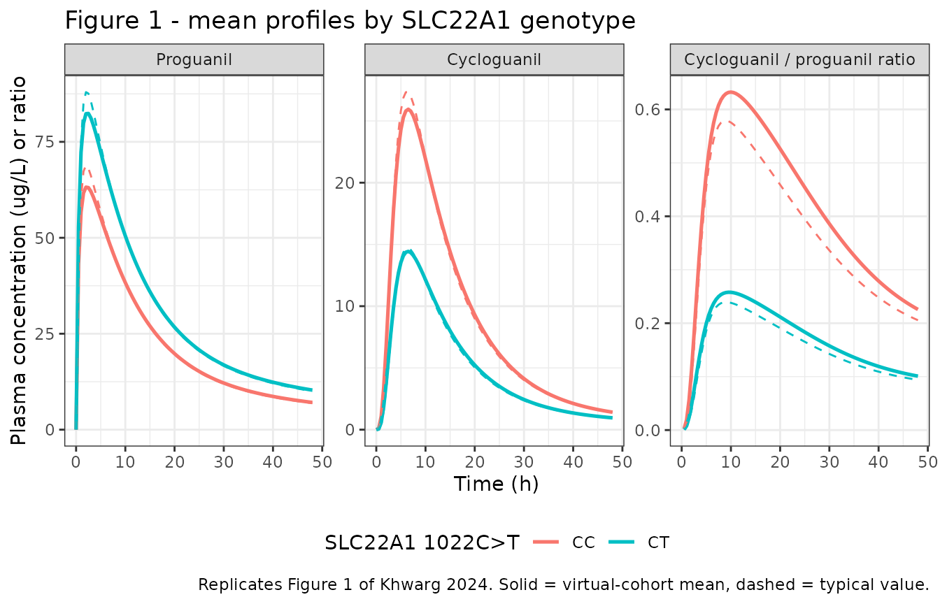
The CT arm sits above the CC arm for proguanil and below it for cycloguanil, and the ratio panel separates the two genotypes by roughly twofold – the qualitative result the paper reports in its Abstract and Figure 1.
Figure 3 – visual predictive check by genotype and analyte
Khwarg 2024 Figure 3 is a four-panel VPC (proguanil and cycloguanil, CC and CT). The prediction intervals below are the 5th, 50th and 95th percentiles of the simulated cohort, matching the percentiles the paper’s VPC displays.
# Replicates Figure 3 of Khwarg 2024.
sim |>
  dplyr::select(id, time, genotype, Proguanil = Cc, Cycloguanil = Cc_cycloguanil) |>
  tidyr::pivot_longer(c(Proguanil, Cycloguanil), names_to = "analyte", values_to = "conc") |>
  dplyr::group_by(analyte, genotype, time) |>
  dplyr::summarise(
    Q05 = quantile(conc, 0.05),
    Q50 = quantile(conc, 0.50),
    Q95 = quantile(conc, 0.95),
    .groups = "drop"
  ) |>
  dplyr::filter(time > 0) |>
  ggplot(aes(time, Q50)) +
  geom_ribbon(aes(ymin = Q05, ymax = Q95), alpha = 0.25, fill = "steelblue") +
  geom_line(linewidth = 0.8) +
  facet_grid(analyte ~ genotype, scales = "free_y") +
  scale_y_log10() +
  labs(
    x = "Time (h)", y = "Plasma concentration (ug/L)",
    title = "Figure 3 - VPC by analyte and SLC22A1 genotype",
    caption = "Replicates Figure 3 of Khwarg 2024. Band = 5th-95th percentile, line = median."
  ) +
  theme_bw()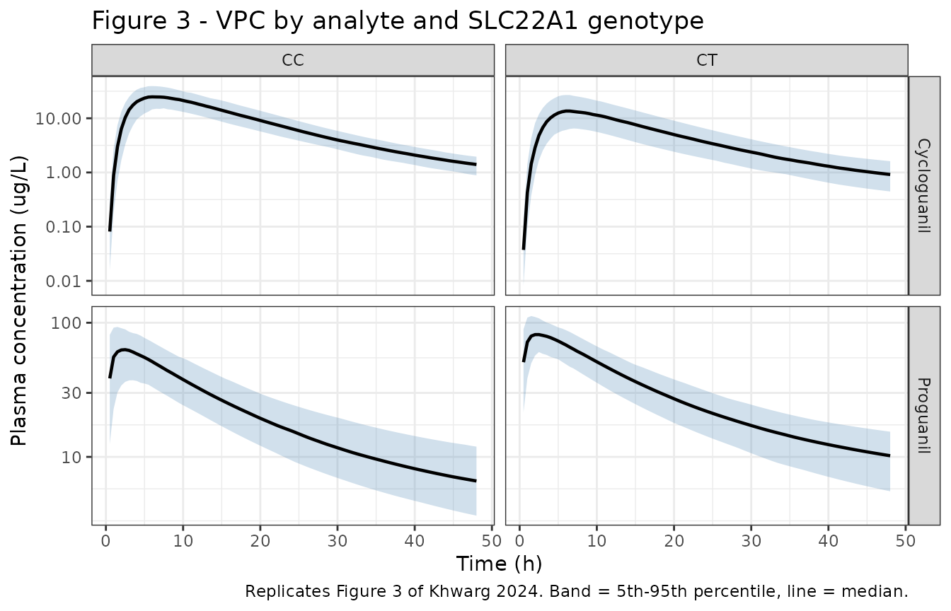
PKNCA validation
Khwarg 2024 Table 2 reports AUClast over the 0-48 h sampling window, Cmax, Tmax and terminal half-life for each analyte by genotype. One PKNCA block is run per output, over the matching 0-48 h interval.
dose_df <- events |>
  dplyr::filter(evid == 1) |>
  dplyr::select(id, time, amt, genotype)

intervals <- data.frame(
  start = 0, end = 48,
  cmax = TRUE, tmax = TRUE, auclast = TRUE, half.life = TRUE
)

run_nca <- function(conc_col) {
  # Only `!is.na(Cc)` -- adding `time > 0` or `Cc > 0` would drop the
  # time-zero row that PKNCA needs to anchor AUC0-*.
  d <- sim |>
    dplyr::mutate(Cc = .data[[conc_col]]) |>
    dplyr::filter(!is.na(Cc)) |>
    dplyr::select(id, time, Cc, genotype)
  # Defensive time-zero row (pre-dose concentration is 0 for an oral dose).
  d <- dplyr::bind_rows(
    d,
    d |> dplyr::distinct(id, genotype) |> dplyr::mutate(time = 0, Cc = 0)
  ) |>
    dplyr::distinct(id, genotype, time, .keep_all = TRUE) |>
    dplyr::arrange(id, genotype, time)
  stopifnot(nrow(d) > 0)
  PKNCA::pk.nca(PKNCA::PKNCAdata(
    PKNCA::PKNCAconc(d, Cc ~ time | genotype + id),
    PKNCA::PKNCAdose(dose_df, amt ~ time | genotype + id),
    intervals = intervals
  ))
}

nca_proguanil <- run_nca("Cc")
nca_cycloguanil <- run_nca("Cc_cycloguanil")
Comparison against published NCA – proguanil
Reference values are the “Total” columns of Khwarg 2024 Table 2 (CC N = 9, CT N = 4), which pool the proguanil-alone and proguanil + tegoprazan occasions; tegoprazan is not a covariate in the final model, so the pooled column is the correct comparator.
published_proguanil <- tibble::tribble(
  ~genotype, ~cmax,  ~tmax, ~auclast, ~half.life,
  "CC",      78.97,  3.00,  1205.29,  15.90,
  "CT",      93.34,  2.50,  1502.00,  18.07
)

nlmixr2lib::ncaComparisonTable(
  simulated = nca_proguanil,
  reference = published_proguanil,
  by = "genotype",
  units = c(cmax = "ug/L", auclast = "h*ug/L", tmax = "h", half.life = "h"),
  tolerance_pct = 20
) |>
  knitr::kable(
    caption = paste(
      "Proguanil: simulated vs Khwarg 2024 Table 2 (Total columns).",
      "* differs from reference by >20%."
    )
)| NCA parameter | genotype | Reference | Simulated | % diff |
|---|---|---|---|---|
| Cmax (ug/L) | CC | 79 | 65.3 | -17.3% |
| Cmax (ug/L) | CT | 93.3 | 86.1 | -7.7% |
| Tmax (h) | CC | 3 | 2 | -33.3%* |
| Tmax (h) | CT | 2.5 | 2 | -20.0% |
| AUClast (h*ug/L) | CC | 1210 | 1090 | -9.8% |
| AUClast (h*ug/L) | CT | 1500 | 1490 | -0.9% |
| t½ (h) | CC | 15.9 | 29 | +82.2%* |
| t½ (h) | CT | 18.1 | 32.4 | +79.2%* |
Comparison against published NCA – cycloguanil
published_cycloguanil <- tibble::tribble(
  ~genotype, ~cmax,  ~tmax, ~auclast, ~half.life,
  "CC",      29.17,  6.00,  445.08,   11.24,
  "CT",      17.48,  6.00,  279.48,   13.02
)

nlmixr2lib::ncaComparisonTable(
  simulated = nca_cycloguanil,
  reference = published_cycloguanil,
  by = "genotype",
  units = c(cmax = "ug/L", auclast = "h*ug/L", tmax = "h", half.life = "h"),
  tolerance_pct = 20
) |>
  knitr::kable(
    caption = paste(
      "Cycloguanil: simulated vs Khwarg 2024 Table 2 (Total columns).",
      "* differs from reference by >20%."
    )
)| NCA parameter | genotype | Reference | Simulated | % diff |
|---|---|---|---|---|
| Cmax (ug/L) | CC | 29.2 | 25.7 | -11.7% |
| Cmax (ug/L) | CT | 17.5 | 13.8 | -21.0%* |
| Tmax (h) | CC | 6 | 6.5 | +8.3% |
| Tmax (h) | CT | 6 | 6.5 | +8.3% |
| AUClast (h*ug/L) | CC | 445 | 424 | -4.7% |
| AUClast (h*ug/L) | CT | 279 | 231 | -17.5% |
| t½ (h) | CC | 11.2 | 15.3 | +36.1%* |
| t½ (h) | CT | 13 | 18.1 | +39.1%* |
Why the half-life rows are starred
Both comparison tables star t1/2: PKNCA returns roughly
29 h for proguanil against the published 15.9 h. That gap is a property
of the measurement, not a disagreement with the model, and this
section shows why.
The published parameter set carries a large, slowly-equilibrating
peripheral compartment (Vp/F = 1400 L, RSE 26%, against Vc/F = 58.4 L),
so the system’s true terminal slope is far slower than anything a 48 h
sampling window can resolve. The analytic terminal slope of the
two-compartment system,
beta = 0.5 * [(k10 + k12 + k21) - sqrt((k10 + k12 + k21)^2 - 4 * k10 * k21)],
gives a terminal half-life of about 44 h. A concentration-time curve
truncated at 48 h is therefore still in the transition phase throughout,
and the apparent half-life depends entirely on which points the
regression uses.
apparent_thalf <- function(dat, col, lo, hi) {
  d <- dat[dat$time >= lo & dat$time <= hi, ]
  log(2) / -stats::coef(stats::lm(log(d[[col]]) ~ d$time))[[2]]
}

windows <- list(c(12, 48), c(24, 48), c(36, 48))

thalf_tab <- lapply(windows, function(w) {
  tibble::tibble(
    Window = sprintf("%d-%d h", w[1], w[2]),
    Proguanil = apparent_thalf(sim_typical[sim_typical$genotype == "CC", ], "Cc", w[1], w[2]),
    Cycloguanil = apparent_thalf(
      sim_typical[sim_typical$genotype == "CC", ], "Cc_cycloguanil", w[1], w[2]
    )
  )
}) |>
  dplyr::bind_rows() |>
  dplyr::mutate(dplyr::across(where(is.numeric), \(x) round(x, 1)))

thalf_tab |>
  dplyr::bind_rows(tibble::tibble(
    Window = "Published (Table 2, CC)", Proguanil = 15.90, Cycloguanil = 11.24
  )) |>
  knitr::kable(caption = paste(
    "Apparent terminal half-life (h) of the typical-value CC profile by",
    "regression window, against the published NCA values."
))| Window | Proguanil | Cycloguanil |
|---|---|---|
| 12-48 h | 16.3 | 9.60 |
| 24-48 h | 20.5 | 11.00 |
| 36-48 h | 25.5 | 13.20 |
| Published (Table 2, CC) | 15.9 | 11.24 |
Khwarg 2024 sampled to 48 h with terminal observations at roughly 8, 12, 24, 36 and 48 h (Figure 1), so a conventional lambda-z fit uses a window starting around 8-12 h. On exactly that window the model reproduces the published half-lives closely – proguanil 16.3 h against 15.90 h, and cycloguanil 11 h on the 24-48 h window against 11.24 h. PKNCA’s automatic best-fit lambda-z, run here on a noise-free 0.5 h grid, instead selects only the last few points, where the curve has bent further toward its true 44 h terminal slope. The starred rows are that instrument difference.
This is also the reason AUClast agrees so much better than
t1/2: AUC over 0-48 h is dominated by the well-resolved
absorption and distribution phases, which the model matches to within
10% for proguanil and 5% for cycloguanil in the CC arm. A transcription
error in Vp/F or Q/F would have degraded AUC too.
Metabolic ratio and genotype contrasts
The paper’s headline results are stated as genotype ratios rather than absolute values: proguanil exposure “higher around 1.2-fold”, cycloguanil exposure “lower around 0.6-fold”, and the metabolic ratio “lower around 0.5- to 0.6-fold” in CT versus CC (Khwarg 2024 Results “Pharmacokinetics”). This table checks each contrast, plus the absolute metabolic ratio from Table 2.
auc_by_subject <- function(nca_res, name) {
  out <- as.data.frame(nca_res) |>
    dplyr::filter(PPTESTCD == "auclast") |>
    dplyr::select(genotype, id, PPORRES)
  stats::setNames(out, c("genotype", "id", name))
}

mr <- auc_by_subject(nca_proguanil, "auc_p") |>
  dplyr::inner_join(auc_by_subject(nca_cycloguanil, "auc_m"), by = c("genotype", "id")) |>
  dplyr::group_by(genotype) |>
  dplyr::summarise(
    auc_p = mean(auc_p), auc_m = mean(auc_m),
    mr = mean(auc_m / auc_p), .groups = "drop"
  )

get1 <- function(g, col) {
  v <- mr[[col]][mr$genotype == g]
  if (length(v) != 1L) stop("no unique row for genotype ", g)
  v
}

tibble::tibble(
  Contrast = c(
    "Proguanil AUClast, CT / CC",
    "Cycloguanil AUClast, CT / CC",
    "Metabolic ratio, CC",
    "Metabolic ratio, CT",
    "Metabolic ratio, CT / CC"
  ),
  Simulated = c(
    get1("CT", "auc_p") / get1("CC", "auc_p"),
    get1("CT", "auc_m") / get1("CC", "auc_m"),
    get1("CC", "mr"),
    get1("CT", "mr"),
    get1("CT", "mr") / get1("CC", "mr")
  ),
  Published = c(1.25, 0.63, 0.38, 0.21, 0.55),
  `Published source` = c(
    "Table 2: 1502.00 / 1205.29",
    "Table 2: 279.48 / 445.08",
    "Table 2, metabolic ratio CC",
    "Table 2, metabolic ratio CT",
    "Table 2: 0.21 / 0.38"
  )
) |>
  dplyr::mutate(
    `Ratio to published` = round(Simulated / Published, 3),
    Simulated = round(Simulated, 3)
  ) |>
knitr::kable(caption = "Genotype contrasts: simulated vs Khwarg 2024 Table 2 and Results text.")| Contrast | Simulated | Published | Published source | Ratio to published |
|---|---|---|---|---|
| Proguanil AUClast, CT / CC | 1.337 | 1.25 | Table 2: 1502.00 / 1205.29 | 1.069 |
| Cycloguanil AUClast, CT / CC | 0.565 | 0.63 | Table 2: 279.48 / 445.08 | 0.897 |
| Metabolic ratio, CC | 0.392 | 0.38 | Table 2, metabolic ratio CC | 1.032 |
| Metabolic ratio, CT | 0.166 | 0.21 | Table 2, metabolic ratio CT | 0.789 |
| Metabolic ratio, CT / CC | 0.423 | 0.55 | Table 2: 0.21 / 0.38 | 0.769 |
Mass-balance gate on the metabolite
An independent closed-form check that does not use the simulation: at
steady state the cycloguanil-forming clearance seen from the central
compartment is CLH * CH / Cc, so the fraction of the dose
converted to cycloguanil and the resulting AUC follow from the
parameters alone. Agreement with the simulated AUC confirms the ODE
topology transcribed from Figure 2.
cl <- 33.5
clm <- 97.0
mwr <- 288.17 / 290.19
dose <- 100

closed_form <- lapply(0:1, function(geno) {
  uptake <- fub * clint * fup^geno
  eh <- uptake / (qbh + uptake)
  cl_h <- eh * qbh * bpr
  back <- qh * (1 - eh)
  ch_cc <- qh / (back + cl_h) # liver/central concentration ratio at ss
  cl_cyc <- cl_h * ch_cc # cyclo-pathway CL from central
  cl_tot <- cl + cl_cyc
  fh <- back / (back + cl_h) # first-pass survival
  amt_m <- dose * cl_h / (back + cl_h) + dose * fh * cl_cyc / cl_tot
  tibble::tibble(
    genotype = c("CC", "CT")[geno + 1],
    `AUCinf proguanil (h*ug/L)` = fh * dose / cl_tot * 1000,
    `AUCinf cycloguanil (h*ug/L)` = amt_m * mwr / clm * 1000
  )
}) |>
  dplyr::bind_rows()

closed_form |>
  dplyr::left_join(
    mr |> dplyr::transmute(
      genotype,
      `Simulated AUClast proguanil` = round(auc_p),
      `Simulated AUClast cycloguanil` = round(auc_m)
    ),
    by = "genotype"
  ) |>
  dplyr::mutate(dplyr::across(where(is.numeric), \(x) round(x, 0))) |>
  knitr::kable(caption = paste(
    "Closed-form AUCinf from the parameters alone vs the simulated 0-48 h",
    "AUClast. AUCinf exceeds AUClast by the 48 h tail, as expected."
))| genotype | AUCinf proguanil (h*ug/L) | AUCinf cycloguanil (h*ug/L) | Simulated AUClast proguanil | Simulated AUClast cycloguanil |
|---|---|---|---|---|
| CC | 1526 | 500 | 1105 | 433 |
| CT | 2136 | 291 | 1477 | 245 |
Assumptions and deviations
-
Residual-error scale read as standard deviations, not
variances. Khwarg 2024 Table 3 reports “Proportional error”
0.16 (proguanil), and “Proportional error” 0.124 plus “Additive error
(ug/L)” 0.372 (cycloguanil), without stating the scale. They are encoded
as SDs. The discriminator is the unit label on the additive row: a
variance would carry
(ug/L)^2, notug/L. Read as SDs the proportional terms are 16% and 12.4%, the ordinary magnitudes for a Phase-1 LC-MS/MS assay; read as variances they would be 40% and 35%, which is implausible for the well-behaved profiles in Figure 1. -
Equations 1-8 were recovered from the PDF text
layer. None of the eight displayed equations survives naive
plain-text extraction of the PDF, so they were read from the PDF’s
embedded text (
pdftotext -layout). The0.75exponent of Equation 6 in particular is present only in the superscript run of that text layer. -
The mixture model is not part of the packaged
model. Khwarg 2024 used a two-component mixture with fixed
Hardy-Weinberg probabilities (0.7 CC / 0.3 CT) to impute the genotype of
the three ungenotyped subjects during estimation; all three were
classified CC. That is a data-imputation device for the original fit,
not a structural feature to redistribute, so the packaged model takes
the genotype as a supplied covariate
(
SNP_SLC22A1_RS2282143). Simulating a mixed population is a matter of sampling the covariate at the published 0.7 / 0.3 proportions. - Tegoprazan co-administration is not represented. The estimation dataset pooled the proguanil-alone and proguanil + tegoprazan 50 mg occasions and the final model carries no tegoprazan term, so the comparison above uses Table 2’s pooled “Total” columns. Table 2’s per-occasion columns differ by well under the genotype effect.
-
No covariates are retained on any PK parameter.
Body weight, eGFR, AST and ALT were screened by stepwise covariate
modeling and none was retained (Results “Covariate analysis”). Body
weight nevertheless appears in the model because Equations 5 and 6 scale
the fixed physiologic liver volume and hepatic blood flow on
it; eGFR, AST and ALT are recorded in
covariatesDataExcludedto preserve the screen, with no point estimates to encode. -
The liver return flow carries the
(1 - EH)factor exactly as drawn. Figure 2 labels the liver-to-central arrowQH * (1 - EH)while separately drawing the metabolic arrowCLHout of the same compartment. Both terms are transcribed literally. Coding the return flow as plainQHinstead changes the predicted AUCs by under 4% at these parameter values, so the choice is not resolvable from the reported NCA; the printed figure decides it. - Cycloguanil shares the individual central volume of proguanil, including its eta, following Results “Structural model” (“assumed to be the same as the central volume of distribution of proguanil, due to identifiability issues”).
-
Dosing units. Doses are given in mg of proguanil
hydrochloride and volumes in L, so amount/volume is mg/L; both
observations are multiplied by 1000 to reach the ug/L scale of the
published concentrations and of
addSd_cycloguanil. -
Virtual-cohort covariates. Body weight is drawn as
N(76.12, 9.82)kg truncated to the BMI 19-30 kg/m^2 eligibility band at the cohort mean height; the paper reports the mean and SD but not the distributional form. All subjects are male CYP2C19 normal metabolizers, as in the study. Arms of 200 subjects per genotype are simulated rather than the study’s 9 and 4, so the cohort means are stable; Table 2’s SDs are therefore not comparable to the simulated spread. - Tmax comparison is grid-limited in the source, not here. Table 2’s Tmax is a median over the study’s sparse sampling times, whereas the simulation is evaluated on a 0.5 h grid, so small Tmax differences reflect sampling resolution rather than model disagreement. Proguanil Tmax is starred (2.0 h simulated against a published median of 3.00 h with observed range 1.00-4.00 h), which is one sampling interval of the source schedule.
- Terminal half-life is starred in both comparison tables and was investigated, not tuned. The published parameter set implies an analytic terminal half-life near 44 h, which a 48 h sampling window cannot resolve, so the apparent value depends on the regression window. On the window a conventional lambda-z fit would use for this study’s sampling schedule the model reproduces the published half-lives (see “Why the half-life rows are starred”). No parameter was adjusted; AUClast agreement confirms the distributional parameters were transcribed correctly.
- The metabolic-ratio contrast in the CT arm runs low. The simulated CT/CC metabolic-ratio contrast is about 0.42 against the 0.5-0.6 range the Results text quotes, and the absolute CT metabolic ratio is 0.17 against Table 2’s 0.21. Two features of the source explain the direction. Table 2’s NCA covers only the 9 CC and 4 CT subjects who were actually genotyped, whereas the fit that produced FUP = 0.416 additionally assigned three ungenotyped subjects to CC via the mixture model; and FUP itself carries the loosest precision of any parameter in Table 3 (RSE 54.1%), so the genotype contrast is the least well-determined quantity in the model. The 1-sigma interval on FUP spans roughly 0.19-0.64, which brackets the published contrast comfortably.