Fosfomycin intrapulmonary PK (Al Hroot 2025)
Source:vignettes/articles/AlHroot_2025_fosfomycin.Rmd
AlHroot_2025_fosfomycin.RmdModel and source
Al Hroot et al. (2025) fitted a minimal physiologically based PK (m-PBPK) model to plasma, epithelial lining fluid (ELF) and alveolar macrophage (AM) concentrations of intravenous fosfomycin (ZTI-01) in healthy adults. They then used it to simulate pneumonia patients and to compute the probability of target attainment (PTA).
- Model:
AlHroot_2025_fosfomycin_pbpk - Description: mPBPK (minimal physiologically based). Intravenous fosfomycin (ZTI-01) in healthy adults: plasma, a lumped residual-tissue compartment, and a lung resolved into interstitial fluid, lung tissue, epithelial lining fluid (ELF) and alveolar macrophages (AMs). The lung interstitial fluid receives the whole cardiac output, the residual tissues a fitted fraction of it; lung tissue and ELF exchange with the interstitial fluid by permeability-surface products and partition coefficients, and drug moves between ELF and AMs by first-order uptake and efflux. Linear elimination from plasma. Physiological volumes and cardiac output are fixed 70 kg values; plasma, ELF and AM concentrations were fitted simultaneously with a single proportional residual error.
- Citation: Al Hroot J, Reeder J, Yuan X, Gu K, Walter E, Boole L, Que L, An G. Determining an appropriate fosfomycin (ZTI-01) dosing regimen in pneumonia patients by utilizing minimal PBPK modeling and target attainment analysis. Antimicrob Agents Chemother. 2025;69(6):e01869-24. doi:10.1128/aac.01869-24.
- Article: https://doi.org/10.1128/aac.01869-24
Population
Thirty-seven healthy adults aged 18-45 years with normal renal function were enrolled in the NIAID Phase 1 intrapulmonary PK study NCT03910673 at the Duke University Early Phase Clinical Research Unit (Methods, “Data source”; Fig. 1). Each received three 6 g doses of intravenous fosfomycin, each infused over 1 h every 8 h. Plasma was sampled before every dose and at 0.5, 1, 1.25, 2 and 5 h after the first and third doses, with extra samples 8 and 12 h after the third dose. Thirty participants had one bronchoalveolar lavage at a randomised time (0.5, 1.25, 2, 5 or 8 h) after the third dose, six per time point, from which the ELF and AM concentrations were measured by LC-MS/MS. The paper gives no weight, sex or race summary. Pneumonia patients were not studied; the paper simulates them by changing two lung parameters (Table 3).
The same information is available programmatically via
readModelDb("AlHroot_2025_fosfomycin_pbpk")()$population.
Source trace
The per-parameter origin is recorded as an in-file comment next to
each ini() entry in
inst/modeldb/specificDrugs/AlHroot_2025_fosfomycin_pbpk.R.
The table below collects them in one place for review.
| Equation / parameter | Value | Source location |
|---|---|---|
d/dt(plasma), d/dt(is_lung),
d/dt(lung), d/dt(elf),
d/dt(alveolar_macrophage), d/dt(other)
|
n/a | Equations 1-6 (Methods, “Final model”); structure in Fig. 2 |
Cc = plasma / v_plasma,
Celf = elf / v_elf,
Calveolar_macrophage = alveolar_macrophage / v_alveolar_macrophage
|
n/a | Not printed; confirmed against the Fig. 3 predicted lines (below) |
qc |
336 L/h (fixed) | Table 1 |
v_plasma, v_other, v_is_lung,
v_lung, v_elf,
v_alveolar_macrophage
|
3, 66, 0.3, 0.7, 0.026, 0.0026 L (fixed) | Table 1 |
lcl |
log(6.59) L/h | Results, “Estimated parameters” (Table 2 prints 7.0; see Assumptions) |
lfq_other (Fd) |
log(0.396) | Table 2 |
lkp_lung, lkp_other, lkp_elf,
lkp_alveolar_macrophage
|
log(11.6), log(0.142), log(0.393), log(0.000023) | Table 2 |
lps_lung (PS1), lps_elf (PS2) |
log(4.55), log(0.0316) L/h | Table 2 |
lk_elf_alveolar_macrophage (K1),
lk_alveolar_macrophage_elf (K2) |
log(0.00515), log(0.000006) 1/h | Table 2 |
etalcl, etalk_alveolar_macrophage_elf
|
12.1 %CV, 40.0 %CV | Table 2, as log(1 + CV^2) |
propSd, propSd_Celf,
propSd_Calveolar_macrophage
|
sqrt(0.0303) | Table 2 sigma^2 (proportional), one value shared by all three matrices |
Pneumonia scenario: lkp_elf, v_elf
|
log(0.29), 0.039 L | Table 3; Methods, “Probability of target attainment” |
Study regimen: three 6 g doses every 8 h
The model has three endpoints (plasma, ELF, AM), so observation rows
name the dosed state and carry dvid = 1; rxode2 returns
every concentration column on each row.
make_events <- function(dose_cmt, doses = c(0, 8, 16), amt = 6000, tgrid) {
  dose <- data.frame(
    id = 1L, time = doses, amt = amt, rate = amt, evid = 1L,
    cmt = dose_cmt, dvid = NA_integer_
  )
  obs <- data.frame(
    id = 1L, time = tgrid, amt = 0, rate = 0, evid = 0L,
    cmt = dose_cmt, dvid = 1L
  )
  dplyr::arrange(dplyr::bind_rows(dose, obs), time, dplyr::desc(evid))
}
tgrid <- sort(unique(c(seq(0, 28, by = 0.05), 17.25)))

mod_pbpk <- readModelDb("AlHroot_2025_fosfomycin_pbpk")
typ_pbpk <- rxode2::rxSolve(rxode2::zeroRe(mod_pbpk), make_events("plasma", tgrid = tgrid)) |>
  as.data.frame()
#> ℹ parameter labels from comments will be replaced by 'label()'
#> ℹ omega/sigma items treated as zero: 'etalcl', 'etalk_alveolar_macrophage_elf'
Figure 3: concentration-time profiles
typ_pbpk |>
  dplyr::select(time, Plasma = Cc, ELF = Celf, AMs = Calveolar_macrophage) |>
  tidyr::pivot_longer(c(Plasma, ELF, AMs), names_to = "matrix", values_to = "conc") |>
  dplyr::filter(matrix == "Plasma" | time >= 16) |>
  dplyr::mutate(matrix = factor(matrix, c("Plasma", "ELF", "AMs"))) |>
  ggplot(aes(time, conc, colour = matrix)) +
  geom_line() +
  facet_wrap(~matrix, scales = "free_x") +
  scale_y_log10(limits = c(1, 1000)) +
  labs(
    x = "Time (h)", y = "Fosfomycin (mg/L)", colour = NULL,
    caption = "Replicates Figure 3 of Al Hroot 2025: 6 g every 8 h, 1-h infusions."
  )
#> Warning in scale_y_log10(limits = c(1, 1000)): log-10 transformation introduced
#> infinite values.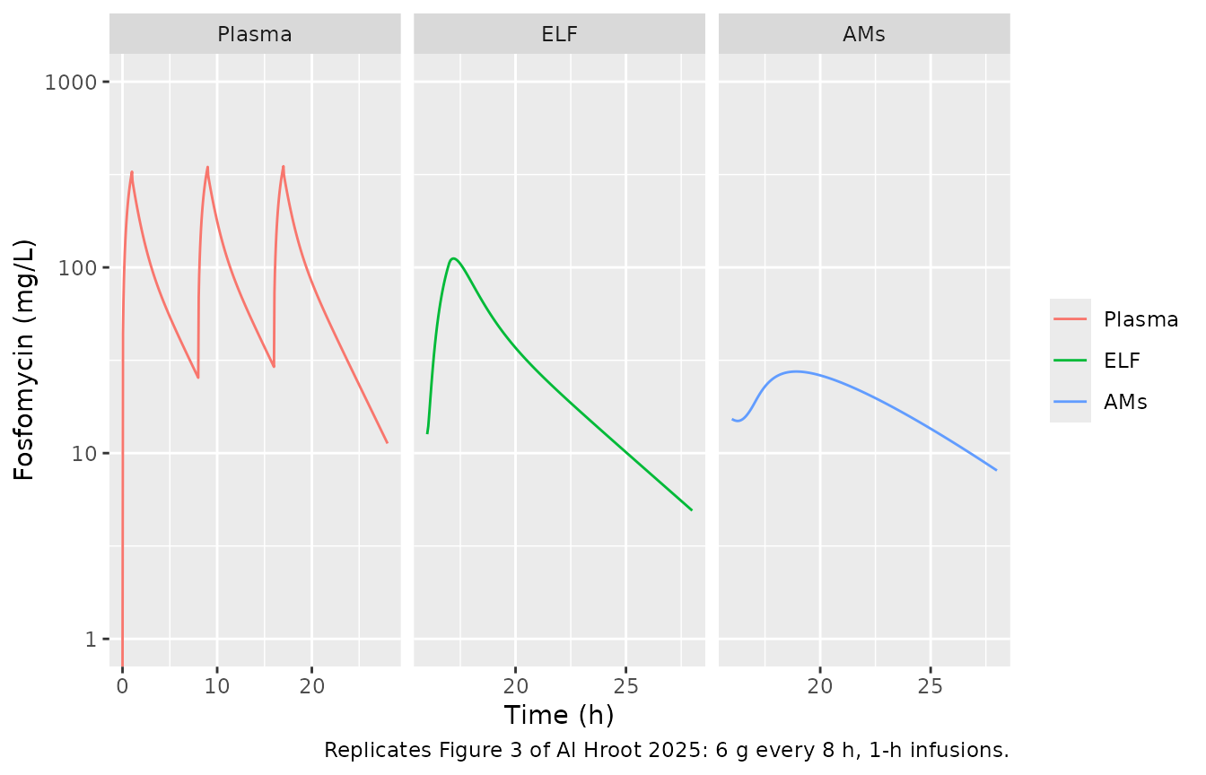
The predicted lines in Fig. 3 are straight segments joining the model
predictions at the sampling times. The maintainers digitised each
segment and read its value at the sampling time it ends on; where a
marker covers that end the segment was extrapolated to it. The dashed AM
line is too faint to resolve point by point, but it stays at about 24
mg/L between its 18 h and 21 h nodes. The table compares the
typical-value predictions with these values. The column
CL 7.0 repeats the prediction with the Table 2 clearance in
place of the Results-text value; see Assumptions.
fig3 <- tibble::tribble(
  ~matrix, ~time, ~fig3,
  "Plasma", 5, 54.5,
  "Plasma", 8, 25.9,
  "Plasma", 16, 29.6,
  "Plasma", 21, 62.2,
  "Plasma", 24, 29.5,
  "Plasma", 28, 11.5,
  "ELF", 18, 80.4,
  "ELF", 21, 26.7,
  "AMs", 18, 24,
  "AMs", 21, 24
)
col_of <- c(Plasma = "Cc", ELF = "Celf", AMs = "Calveolar_macrophage")
pred_at <- function(sim, matrix, time) {
  v <- vapply(seq_along(matrix), function(i) {
    row <- sim[abs(sim$time - time[i]) < 1e-8, col_of[[matrix[i]]]]
    if (length(row) != 1L) stop("no unique prediction at t = ", time[i])
    row
  }, numeric(1))
  v
}
typ_cl7 <- rxode2::rxSolve(
  rxode2::zeroRe(mod_pbpk) |> rxode2::ini(lcl = log(7.0)),
  make_events("plasma", tgrid = tgrid)
) |>
  as.data.frame()
#> ℹ parameter labels from comments will be replaced by 'label()'
#> ℹ change initial estimate of `lcl` to `1.94591014905531`
#> ℹ omega/sigma items treated as zero: 'etalcl', 'etalk_alveolar_macrophage_elf'

fig3_cmp <- fig3 |>
  dplyr::mutate(
    pbpk = pred_at(typ_pbpk, matrix, time),
    pbpk_cl7 = pred_at(typ_cl7, matrix, time),
    pct_pbpk = 100 * (pbpk / fig3 - 1),
    pct_pbpk_cl7 = 100 * (pbpk_cl7 / fig3 - 1)
  )
fig3_cmp |>
  dplyr::select(
    Matrix = matrix, "Time (h)" = time, "Fig. 3 line (mg/L)" = fig3,
    "Model (mg/L)" = pbpk, "% diff" = pct_pbpk,
    "CL 7.0 (mg/L)" = pbpk_cl7, "CL 7.0 % diff" = pct_pbpk_cl7
  ) |>
knitr::kable(digits = 1, caption = "Typical-value predictions against the digitised Fig. 3 lines.")| Matrix | Time (h) | Fig. 3 line (mg/L) | Model (mg/L) | % diff | CL 7.0 (mg/L) | CL 7.0 % diff |
|---|---|---|---|---|---|---|
| Plasma | 5 | 54.5 | 54.2 | -0.5 | 49.5 | -9.2 |
| Plasma | 8 | 25.9 | 25.5 | -1.6 | 22.5 | -13.1 |
| Plasma | 16 | 29.6 | 29.2 | -1.5 | 25.5 | -13.8 |
| Plasma | 21 | 62.2 | 62.9 | 1.1 | 56.7 | -8.8 |
| Plasma | 24 | 29.5 | 29.7 | 0.6 | 25.9 | -12.2 |
| Plasma | 28 | 11.5 | 11.3 | -2.0 | 9.4 | -17.9 |
| ELF | 18 | 80.4 | 83.5 | 3.9 | 79.9 | -0.6 |
| ELF | 21 | 26.7 | 27.5 | 3.0 | 24.9 | -6.7 |
| AMs | 18 | 24.0 | 25.8 | 7.6 | 24.6 | 2.7 |
| AMs | 21 | 24.0 | 23.9 | -0.6 | 22.5 | -6.4 |
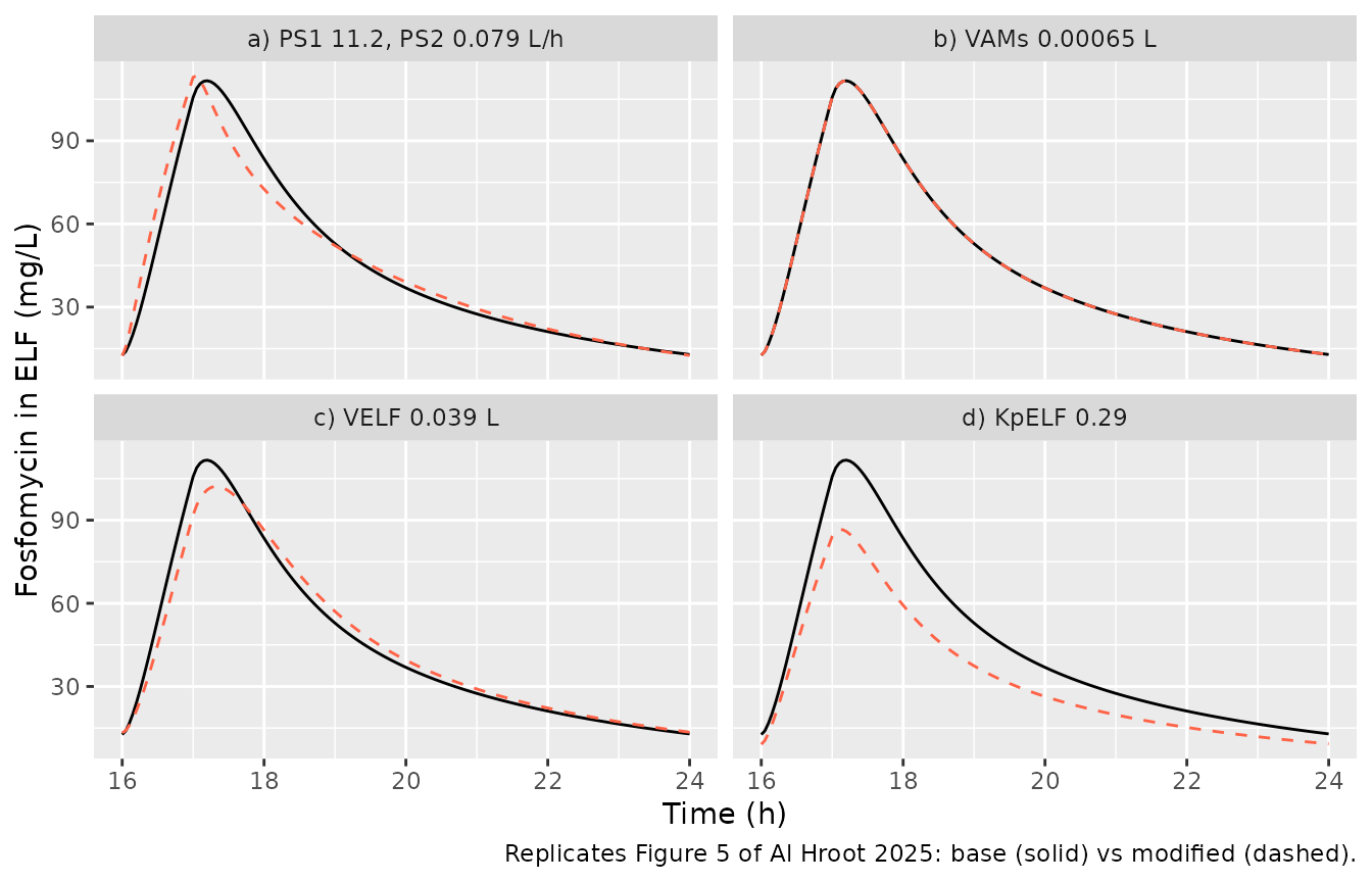
Sensitivity analysis: pneumonia-related changes (Figure 5, Table 3)
Table 3 changes one lung parameter at a time from its healthy value. The profiles below are typical-value ELF concentrations after the third 6 g dose.
scen <- list(
  "Base model" = mod_pbpk,
  "a) PS1 11.2, PS2 0.079 L/h" = mod_pbpk |> rxode2::ini(lps_lung = log(11.2), lps_elf = log(0.079)),
  "b) VAMs 0.00065 L" = mod_pbpk |> rxode2::ini(v_alveolar_macrophage = 0.00065),
  "c) VELF 0.039 L" = mod_pbpk |> rxode2::ini(v_elf = 0.039),
  "d) KpELF 0.29" = mod_pbpk |> rxode2::ini(lkp_elf = log(0.29))
)
#> ℹ parameter labels from comments will be replaced by 'label()'
#> ℹ change initial estimate of `lps_lung` to `2.41591377830105`
#> ℹ change initial estimate of `lps_elf` to `-2.53830742651512`
#> ℹ parameter labels from comments will be replaced by 'label()'
#> ℹ change initial estimate of `v_alveolar_macrophage` to `0.00065`
#> ℹ parameter labels from comments will be replaced by 'label()'
#> ℹ change initial estimate of `v_elf` to `0.039`
#> ℹ parameter labels from comments will be replaced by 'label()'
#> ℹ change initial estimate of `lkp_elf` to `-1.23787435600162`
sens <- dplyr::bind_rows(lapply(names(scen), function(nm) {
  rxode2::rxSolve(rxode2::zeroRe(scen[[nm]]), make_events("plasma", tgrid = tgrid)) |>
    as.data.frame() |>
    dplyr::mutate(scenario = nm)
}))
#> ℹ parameter labels from comments will be replaced by 'label()'
#> ℹ omega/sigma items treated as zero: 'etalcl', 'etalk_alveolar_macrophage_elf'
#> ℹ omega/sigma items treated as zero: 'etalcl', 'etalk_alveolar_macrophage_elf'
#> ℹ omega/sigma items treated as zero: 'etalcl', 'etalk_alveolar_macrophage_elf'
#> ℹ omega/sigma items treated as zero: 'etalcl', 'etalk_alveolar_macrophage_elf'
#> ℹ omega/sigma items treated as zero: 'etalcl', 'etalk_alveolar_macrophage_elf'
base_line <- sens |>
  dplyr::filter(scenario == "Base model") |>
  dplyr::select(time, Celf_base = Celf)
sens |>
  dplyr::filter(scenario != "Base model", time >= 16, time <= 24) |>
  dplyr::left_join(base_line, by = "time") |>
  ggplot(aes(time)) +
  geom_line(aes(y = Celf_base), colour = "black") +
  geom_line(aes(y = Celf), colour = "tomato", linetype = "dashed") +
  facet_wrap(~scenario) +
  labs(
    x = "Time (h)", y = "Fosfomycin in ELF (mg/L)",
    caption = "Replicates Figure 5 of Al Hroot 2025: base (solid) vs modified (dashed)."
  )
sens_tab <- sens |>
  dplyr::filter(time >= 16, time <= 24) |>
  dplyr::group_by(scenario) |>
  dplyr::summarise(
    elf_cmax = max(Celf),
    elf_auc = sum(diff(time) * (head(Celf, -1) + tail(Celf, -1)) / 2),
    plasma_auc = sum(diff(time) * (head(Cc, -1) + tail(Cc, -1)) / 2),
    .groups = "drop"
  ) |>
  dplyr::mutate(
    pct_elf_cmax = 100 * (elf_cmax / elf_cmax[scenario == "Base model"] - 1),
    pct_elf_auc = 100 * (elf_auc / elf_auc[scenario == "Base model"] - 1),
    pct_plasma_auc = 100 * (plasma_auc / plasma_auc[scenario == "Base model"] - 1)
  )
sens_tab |>
  dplyr::select(
    Scenario = scenario, "ELF Cmax (mg/L)" = elf_cmax,
    "ELF Cmax % change" = pct_elf_cmax, "ELF AUC16-24 % change" = pct_elf_auc,
    "Plasma AUC16-24 % change" = pct_plasma_auc
  ) |>
knitr::kable(digits = 1, caption = "Effect of each Table 3 change on the third-dose ELF and plasma exposure.")| Scenario | ELF Cmax (mg/L) | ELF Cmax % change | ELF AUC16-24 % change | Plasma AUC16-24 % change |
|---|---|---|---|---|
| Base model | 111.7 | 0.0 | 0.0 | 0.0 |
| a) PS1 11.2, PS2 0.079 L/h | 113.5 | 1.6 | 0.2 | 0.1 |
| b) VAMs 0.00065 L | 111.7 | 0.0 | 0.0 | 0.0 |
| c) VELF 0.039 L | 102.2 | -8.5 | 0.0 | 0.0 |
| d) KpELF 0.29 | 86.7 | -22.4 | -26.2 | 0.0 |
pct <- function(nm, col) {
  v <- sens_tab[[col]][sens_tab$scenario == nm]
  if (length(v) != 1L) stop("no unique row for '", nm, "'")
  v
}
# Table 3 / Results: no change alters plasma; VAMs has no effect on the ELF;
# VELF lowers it slightly; KpELF has the greatest effect.
stopifnot(
  all(abs(sens_tab$pct_plasma_auc) < 1),
  abs(pct("b) VAMs 0.00065 L", "pct_elf_auc")) < 1,
  pct("c) VELF 0.039 L", "pct_elf_cmax") < 0,
  pct("d) KpELF 0.29", "pct_elf_auc") < -15,
  abs(pct("d) KpELF 0.29", "pct_elf_auc")) > abs(pct("c) VELF 0.039 L", "pct_elf_auc"))
)
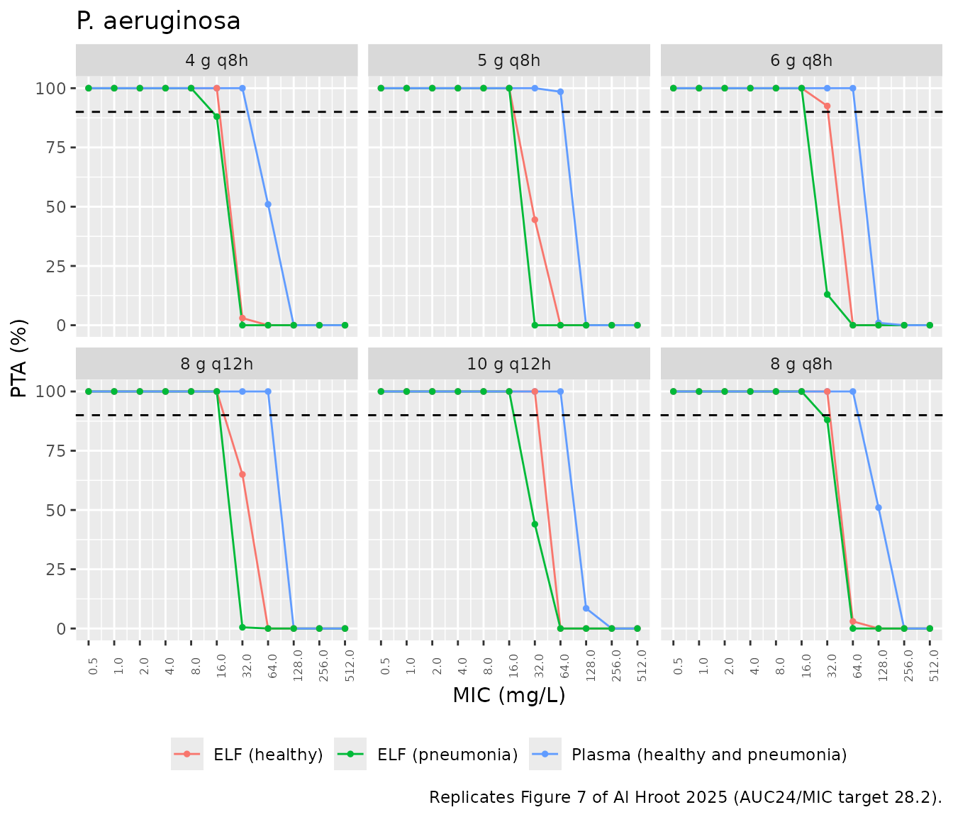
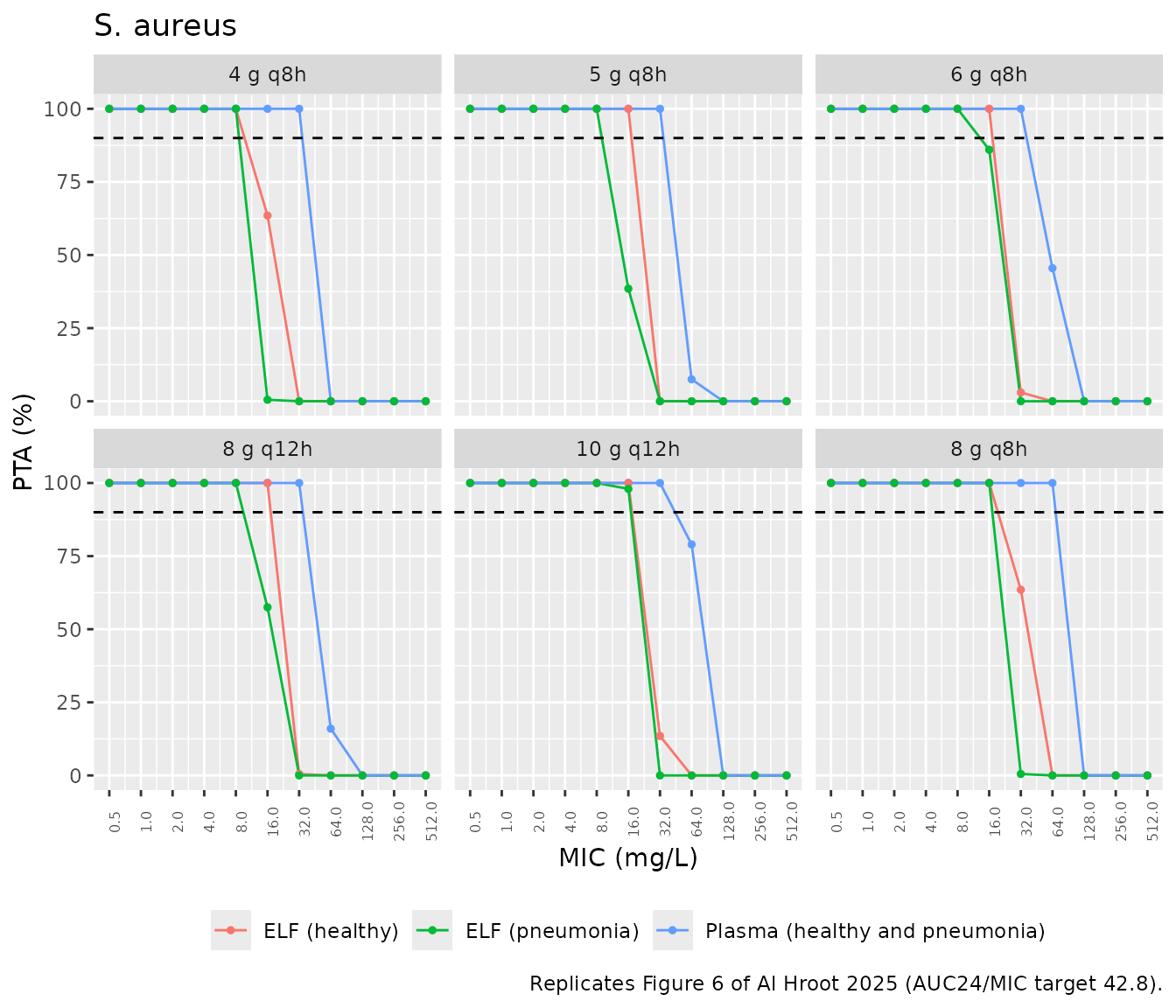
Probability of target attainment (Figures 6 and 7, Table 4)
The paper simulated 1,000 subjects per scenario at steady state for 4, 5, 6 and 8 g every 8 h and 8 and 10 g every 12 h, all as 1-h infusions, and scored AUC24/MIC against 28.2 (P. aeruginosa) and 42.8 (S. aureus). The model is linear and every regimen uses the same 1-h infusion, so the steady-state AUC24 of any regimen is the daily dose times the single-dose AUC0-inf per gram. Below, 200 virtual subjects per population each receive one 1 g dose, PKNCA computes their plasma and ELF AUC, and the regimens are formed by that scaling. The pneumonia population uses KpELF = 0.29 and VELF = 0.039 L, as in the paper; its plasma exposure is identical to that of healthy subjects.
rxode2::rxSetSeed(20250603)
n_per_pop <- 200L
pta_grid <- sort(unique(c(seq(0, 4, by = 0.1), seq(4, 24, by = 0.5), seq(24, 72, by = 1))))
pop_models <- list(
  Healthy = mod_pbpk,
  Pneumonia = mod_pbpk |> rxode2::ini(lkp_elf = log(0.29), v_elf = 0.039)
)
#> ℹ parameter labels from comments will be replaced by 'label()'
#> ℹ change initial estimate of `lkp_elf` to `-1.23787435600162`
#> ℹ change initial estimate of `v_elf` to `0.039`
pta_sim <- dplyr::bind_rows(lapply(seq_along(pop_models), function(i) {
  ev <- make_events("plasma", doses = 0, amt = 1000, tgrid = pta_grid)
  ev <- dplyr::bind_rows(lapply(seq_len(n_per_pop), function(j) dplyr::mutate(ev, id = (i - 1L) * n_per_pop + j)))
  rxode2::rxSolve(pop_models[[i]], ev) |>
    as.data.frame() |>
    dplyr::mutate(population = names(pop_models)[i])
}))
#> ℹ parameter labels from comments will be replaced by 'label()'
stopifnot(dplyr::n_distinct(pta_sim$id) == 2L * n_per_pop)
PKNCA
nca_one <- function(sim, conc_col, matrix_label) {
  conc <- sim |>
    dplyr::transmute(id, population, time, conc = .data[[conc_col]]) |>
    dplyr::filter(!is.na(conc))
  stopifnot(all(conc$conc >= -1e-6 * max(conc$conc)))
  conc <- dplyr::mutate(conc, conc = pmax(conc, 0))
  dose <- sim |>
    dplyr::distinct(id, population) |>
    dplyr::mutate(time = 0, amt = 1000)
  res <- PKNCA::pk.nca(PKNCA::PKNCAdata(
    PKNCA::PKNCAconc(conc, conc ~ time | population + id),
    PKNCA::PKNCAdose(dose, amt ~ time | population + id),
    intervals = data.frame(start = 0, end = Inf, cmax = TRUE, tmax = TRUE, auclast = TRUE, aucinf.obs = TRUE)
  ))
  as.data.frame(res) |>
    dplyr::mutate(matrix = matrix_label)
}
nca <- dplyr::bind_rows(
  nca_one(pta_sim, "Cc", "Plasma"),
  nca_one(pta_sim, "Celf", "ELF")
)
nca |>
  dplyr::group_by(matrix, population, PPTESTCD) |>
  dplyr::summarise(median = median(PPORRES), .groups = "drop") |>
  tidyr::pivot_wider(names_from = PPTESTCD, values_from = median) |>
  dplyr::select(
    Matrix = matrix, Population = population, "Cmax (mg/L)" = cmax,
    "Tmax (h)" = tmax, "AUClast (mg*h/L)" = auclast, "AUCinf (mg*h/L)" = aucinf.obs
  ) |>
knitr::kable(digits = 2, caption = "Median single-dose (1 g, 1-h infusion) NCA by matrix and population.")| Matrix | Population | Cmax (mg/L) | Tmax (h) | AUClast (mg*h/L) | AUCinf (mg*h/L) |
|---|---|---|---|---|---|
| ELF | Healthy | 17.00 | 1.2 | 59.18 | 59.18 |
| ELF | Pneumonia | 12.29 | 1.2 | 44.30 | 44.30 |
| Plasma | Healthy | 54.52 | 1.0 | 150.56 | 150.56 |
| Plasma | Pneumonia | 54.71 | 1.0 | 152.74 | 152.74 |
# Plasma AUCinf must equal dose / CL for each subject: the same drawn
# parameters feed both sides, so only integration and trapezoid error remain.
cl_i <- pta_sim |>
  dplyr::distinct(id, cl)
auc_chk <- nca |>
  dplyr::filter(matrix == "Plasma", PPTESTCD == "aucinf.obs") |>
  dplyr::left_join(cl_i, by = "id") |>
  dplyr::mutate(ratio = PPORRES / (1000 / cl))
stopifnot(nrow(auc_chk) == 2L * n_per_pop, max(abs(auc_chk$ratio - 1)) < 0.01)
The paper reports no NCA values for these regimens, so there is no published NCA table to compare against; the PTA breakpoints of Table 4 are the published comparison.
regimens <- tibble::tribble(
  ~regimen, ~daily_g,
  "4 g q8h", 12,
  "5 g q8h", 15,
  "6 g q8h", 18,
  "8 g q12h", 16,
  "10 g q12h", 20,
  "8 g q8h", 24
)
targets <- c("P. aeruginosa" = 28.2, "S. aureus" = 42.8)
mics <- 2^(-1:9)
auc1 <- nca |>
  dplyr::filter(PPTESTCD == "aucinf.obs") |>
  dplyr::select(id, population, matrix, auc1g = PPORRES)
pta <- tidyr::expand_grid(
  auc1 |> dplyr::distinct(population, matrix),
  regimens,
  pathogen = names(targets),
  mic = mics
) |>
  dplyr::rowwise() |>
  dplyr::mutate(pta = {
    a <- auc1$auc1g[auc1$population == population & auc1$matrix == matrix]
    100 * mean(a * daily_g / mic >= targets[[pathogen]])
  }) |>
  dplyr::ungroup() |>
  dplyr::mutate(
    curve = ifelse(matrix == "Plasma", "Plasma (healthy and pneumonia)", paste0("ELF (", tolower(population), ")"))
  ) |>
  dplyr::filter(!(matrix == "Plasma" & population == "Pneumonia"))
for (pg in names(targets)) {
  p <- pta |>
    dplyr::filter(pathogen == pg) |>
    dplyr::mutate(regimen = factor(regimen, regimens$regimen)) |>
    ggplot(aes(mic, pta, colour = curve)) +
    geom_line() +
    geom_point(size = 1) +
    geom_hline(yintercept = 90, linetype = "dashed") +
    scale_x_continuous(trans = "log2", breaks = mics) +
    facet_wrap(~regimen) +
    labs(
      x = "MIC (mg/L)", y = "PTA (%)", colour = NULL,
      title = pg,
      caption = sprintf(
        "Replicates Figure %d of Al Hroot 2025 (AUC24/MIC target %s).",
        if (pg == "S. aureus") 6L else 7L, targets[[pg]]
      )
    ) +
    theme(legend.position = "bottom", axis.text.x = element_text(angle = 90, size = 6))
  print(p)
}
breakpoint <- function(x_mic, x_pta) {
  ok <- x_mic[x_pta >= 90]
  if (length(ok) == 0L) NA_real_ else max(ok)
}
bp_sim <- pta |>
  dplyr::group_by(curve, regimen, pathogen) |>
  dplyr::summarise(bp = breakpoint(mic, pta), .groups = "drop")
table4 <- tibble::tribble(
  ~regimen, ~pathogen, ~plasma, ~elf_healthy, ~elf_pneumonia,
  "4 g q8h", "P. aeruginosa", 32, 16, 16,
  "4 g q8h", "S. aureus", 32, 8, 8,
  "5 g q8h", "P. aeruginosa", 64, 16, 16,
  "5 g q8h", "S. aureus", 32, 16, 8,
  "8 g q12h", "P. aeruginosa", 64, 16, 16,
  "8 g q12h", "S. aureus", 32, 16, 8,
  "6 g q8h", "P. aeruginosa", 64, 32, 16,
  "6 g q8h", "S. aureus", 32, 16, 8,
  "10 g q12h", "P. aeruginosa", 64, 32, 16,
  "10 g q12h", "S. aureus", 32, 16, 16,
  "8 g q8h", "P. aeruginosa", 64, 32, 32,
  "8 g q8h", "S. aureus", 64, 16, 16
) |>
  tidyr::pivot_longer(c(plasma, elf_healthy, elf_pneumonia), names_to = "curve", values_to = "bp_paper") |>
  dplyr::mutate(curve = dplyr::recode(curve,
    plasma = "Plasma (healthy and pneumonia)",
    elf_healthy = "ELF (healthy)",
    elf_pneumonia = "ELF (pneumonia)"
  ))
bp_cmp <- dplyr::left_join(table4, bp_sim, by = c("regimen", "pathogen", "curve"))
stopifnot(nrow(bp_cmp) == 36L, !anyNA(bp_cmp$bp))
bp_cmp |>
  dplyr::mutate(cell = sprintf("%g (%g)", bp, bp_paper)) |>
  dplyr::select(regimen, pathogen, curve, cell) |>
  tidyr::pivot_wider(names_from = curve, values_from = cell) |>
  dplyr::rename(Regimen = regimen, Pathogen = pathogen) |>
knitr::kable(caption = "PTA >= 90% breakpoints (mg/L): simulated, with the Table 4 value of Al Hroot 2025 in parentheses.")| Regimen | Pathogen | Plasma (healthy and pneumonia) | ELF (healthy) | ELF (pneumonia) |
|---|---|---|---|---|
| 4 g q8h | P. aeruginosa | 32 (32) | 16 (16) | 8 (16) |
| 4 g q8h | S. aureus | 32 (32) | 8 (8) | 8 (8) |
| 5 g q8h | P. aeruginosa | 64 (64) | 16 (16) | 16 (16) |
| 5 g q8h | S. aureus | 32 (32) | 16 (16) | 8 (8) |
| 8 g q12h | P. aeruginosa | 64 (64) | 16 (16) | 16 (16) |
| 8 g q12h | S. aureus | 32 (32) | 16 (16) | 8 (8) |
| 6 g q8h | P. aeruginosa | 64 (64) | 32 (32) | 16 (16) |
| 6 g q8h | S. aureus | 32 (32) | 16 (16) | 8 (8) |
| 10 g q12h | P. aeruginosa | 64 (64) | 32 (32) | 16 (16) |
| 10 g q12h | S. aureus | 32 (32) | 16 (16) | 16 (16) |
| 8 g q8h | P. aeruginosa | 64 (64) | 32 (32) | 16 (32) |
| 8 g q8h | S. aureus | 64 (64) | 16 (16) | 16 (16) |
n_match <- bp_cmp |>
  dplyr::group_by(is_plasma = grepl("^Plasma", curve)) |>
  dplyr::summarise(match = sum(bp == bp_paper), n = dplyr::n(), .groups = "drop")
n_match
#> # A tibble: 2 × 3
#>   is_plasma match     n
#>   <lgl>     <int> <int>
#> 1 FALSE        22    24
#> 2 TRUE         12    12
# Plasma breakpoints rest on the 10th percentile of dose/CL, at least 5
# binomial standard errors from every MIC boundary with 200 subjects: all 12
# matched at every seed tried. ELF cells for 6 g q8h and 4 g q8h sit on a
# boundary; 10-12 of 12 per population matched across seeds, so the gate is 20
# of 24. A wrong KpELF, PS2 or clearance shifts whole columns.
stopifnot(
  n_match$match[n_match$is_plasma] == 12L,
  n_match$match[!n_match$is_plasma] >= 20L
)
Assumptions and deviations
-
Clearance: 6.59 L/h, not the 7.0 L/h of Table 2.
The Results text says “the systematic clearance was estimated to be 6.59
L/h”, while Table 2 prints CL = 7.0 (RSE 1.9%). There is no confidence
interval to say which is the point estimate, so the maintainers checked
both against the paper’s own outputs. In the Fig. 3 comparison above,
the plasma troughs at 8, 16, 24 and 28 h are within 2% of the digitised
line with 6.59 L/h and 12-18% below it with 7.0 L/h. They are still
9-13% below with 7.0 L/h when the line is taken as the mean of 2,000
individual predictions rather than the typical value. With 1,000
subjects per scenario, 35 of the 36 Table 4 breakpoints come out right
with 6.59 L/h and 33 of 36 with 7.0 L/h. To use the tabulated value, run
mod |> rxode2::ini(lcl = log(7.0)). -
Observed concentrations are amount over volume. The
paper does not print observation equations. The ELF and AM
concentrations are taken as the compartment amount divided by
v_elfandv_alveolar_macrophage, without the partition coefficient; this reproduces the ELF and AM lines of Fig. 3 (table above). -
One residual variance for three matrices. The paper
estimates a single proportional sigma^2 for plasma, ELF and AM data.
nlmixr2 needs a separate parameter for each endpoint, so the same value
is stored three times (
propSd,propSd_Celf,propSd_Calveolar_macrophage). Constrain them to be equal when re-fitting. - IIV CV% converted with omega^2 = log(1 + CV^2). The tables report IIV as %CV.
- PTA by superposition, IIV only. The steady-state AUC24 is computed from a single-dose AUC0-inf scaled by the daily dose (exact for this linear model with a fixed 1-h infusion). Residual error is not added to the simulated concentrations; the paper does not say whether its NONMEM simulation added it. The vignette uses 200 subjects per population rather than 1,000.
- The supplement’s compartmental model is not included. Before the m-PBPK model, the authors built a four-compartment model (central, peripheral, ELF, AMs; supplement Fig. S1, Table S1 model 5, final estimates in Table S2). They replaced it with the m-PBPK model and used only the m-PBPK model for the sensitivity and PTA analyses, so only the final model is packaged. Also, the printed Table S2 values do not reproduce that model’s own diagnostics. Using the Fig. S1 structure (central-ELF k13/k31 and ELF-AM k34/k43 acting on amounts, ELF and AM volumes fixed at 0.026 and 0.0026 L), the plasma and ELF profiles match Fig. 3. The AM concentrations, however, come out at 5-10 mg/L after the third dose. That is about one-third of the 15-35 mg/L population predictions in the AM points of Fig. S2 and of the observed AM data.
-
Compartment names. The plasma, lung interstitial
fluid, lung tissue, ELF and residual tissues use the library’s
registered names
plasma,is_lung,lung,elfandother. The alveolar macrophage state,alveolar_macrophage, is model-specific because the library has no registered name for it. - No erratum was found for this article (checked 2026-11-04).