Ciprofloxacin (Guo 2022)
Source:vignettes/articles/Guo_2022_ciprofloxacin.Rmd
Guo_2022_ciprofloxacin.RmdModel and source
- Citation: Guo T, Abdulla A, Koch BCP, van Hasselt JGC, Endeman H, Schouten JA, Elbers PWG, Bruggemann RJM, van Hest RM; Dutch Antibiotic PK/PD Collaborators. Pooled Population Pharmacokinetic Analysis for Exploring Ciprofloxacin Pharmacokinetic Variability in Intensive Care Patients. Clin Pharmacokinet. 2022;61:869-879. doi:10.1007/s40262-022-01114-5
- Description: Two-compartment population PK model for intravenous ciprofloxacin in critically ill adult ICU patients, developed on individual data pooled from three Dutch ICU studies (Guo 2022). First-order elimination from the central compartment; total body weight enters all four structural parameters allometrically (exponent 0.75 on CL and Q, 1 on V1 and V2, reference 70 kg) and MDRD eGFR enters CL as a linear effect centered on 58.64 mL/min/1.73 m^2. IIV on CL, V1 and V2, inter-occasion variability on CL with one occasion per 24 h of therapy, and a study-specific residual error (combined additive + proportional for study 1, proportional for studies 2 and 3).
- Article: https://doi.org/10.1007/s40262-022-01114-5 (open access)
Population
Guo et al. (2022) pooled individual data from three prospective Dutch
ICU studies of intravenous ciprofloxacin: 1094 total plasma
concentrations from 140 critically ill adults. Study 1 (Erasmus MC and
Maasstad Hospital, Rotterdam; 42 patients, 204 samples) was previously
published as Abdulla 2020 (the EXPAT study; see
Abdulla_2020_ciprofloxacin), study 2 (Radboud UMC,
Nijmegen; 39 patients, 531 samples) as Gieling 2020, and study 3
(Amsterdam UMC location VUmc, the Right Dose Right Now study; 59
patients, 359 samples) was unpublished. Patients were 66% male, median
age 67 years (IQR 59-74), weight 80 kg (IQR 69-93), MDRD eGFR 59
mL/min/1.73 m^2 (IQR 37-96), albumin 25 g/L and SOFA score 10; 8% were
on continuous veno-venous hemofiltration (source Table 1). Most patients
received 400 mg twice or three times daily as 30-60 min infusions; study
3 also used model-based individualized dosing.
The same information is available programmatically via
readModelDb("Guo_2022_ciprofloxacin")()$population.
Age, sex, serum creatinine, eGFR, albumin, SOFA score and CVVH were
screened in a stepwise covariate search. Only eGFR on clearance was
retained, on top of the a priori allometric weight scaling of all four
structural parameters. The screened covariates are recorded in the
model’s covariatesDataExcluded metadata.
Source trace
| Equation / parameter | Value | Source location |
|---|---|---|
lcl (CL) |
log(14.7 L/h) | Table 2, final model; Eq. 3 |
lvc (V1) |
log(61.2 L) | Table 2, final model; Eq. 4 |
lq (Q) |
log(44.9 L/h) | Table 2, final model; Eq. 5 |
lvp (V2) |
log(71.6 L) | Table 2, final model; Eq. 6 |
e_wt_cl, e_wt_q
|
fixed 0.75 | Methods 2.2.2 (a priori allometry); Eqs. 3 and 5 |
e_wt_vc, e_wt_vp
|
fixed 1 | Methods 2.2.2; Eqs. 4 and 6 |
e_crcl_cl |
0.008 per mL/min/1.73 m^2 | Table 2 ‘eGFR on CL (linear)’; Eq. 3 |
| eGFR centre 58.64 mL/min/1.73 m^2 | n/a | Eq. 3; Results 3.1 (median eGFR) |
| Reference weight 70 kg | n/a | Eqs. 3-6 |
etalcl |
0.2011 | Table 2, IIV CL 47.2% -> log(1 + 0.472^2) |
etalvc |
0.3172 | Table 2, IIV V1 61.1% -> log(1 + 0.611^2) |
etalvp |
0.1981 | Table 2, IIV V2 46.8% -> log(1 + 0.468^2) |
etaiov_cl_1 … etaiov_cl_7
|
0.01833 | Table 2, IOV CL 13.6% -> log(1 + 0.136^2); 24-h occasions, Methods 2.2.1 |
propSd (study 2) |
0.137 | Table 2, Prop Study2 13.7% |
propSd_expat, addSd_expat (study 1) |
0.175, 0.151 mg/L | Table 2, Prop Study1 17.5%, Add Study1 0.151 mg/L |
propSd_rdrn (study 3) |
0.245 | Table 2, Prop Study3 24.5% |
| Two-compartment model, first-order elimination | n/a | Results 3.1 |
cl <- ... * (1 + e_crcl_cl * (CRCL - 58.64)) * exp(etalcl + iov_cl) |
n/a | Eq. 3 |
Typical-patient profiles
The typical patient of Equations 3-6 weighs 70 kg and has eGFR 58.64 mL/min/1.73 m^2. Profiles below are for 400 mg every 8 h given as a 30-min infusion, with the random effects removed, across the eGFR range of the pooled cohort.
mod <- readModelDb("Guo_2022_ciprofloxacin")
mod_typ <- rxode2::zeroRe(mod)
#> ℹ parameter labels from comments will be replaced by 'label()'
#> Warning: some etas defaulted to non-mu referenced, possible parsing error: etaiov_cl_1, etaiov_cl_2, etaiov_cl_3, etaiov_cl_4, etaiov_cl_5, etaiov_cl_6, etaiov_cl_7
#> as a work-around try putting the mu-referenced expression on a simple line
#> Warning: No sigma parameters in the model
#> Warning: some etas defaulted to non-mu referenced, possible parsing error: etaiov_cl_1, etaiov_cl_2, etaiov_cl_3, etaiov_cl_4, etaiov_cl_5, etaiov_cl_6, etaiov_cl_7
#> as a work-around try putting the mu-referenced expression on a simple line

typ_subj <- tibble(
  id = 1:4,
  WT = 70,
  CRCL = c(20, 58.64, 100, 140),
  STUDY_EXPAT = 0,
  STUDY_RDRN = 0,
  OCC = 1
)
typ_events <- bind_rows(
  typ_subj |> tidyr::crossing(time = c(0, 8, 16)) |>
    mutate(evid = 1L, amt = 400, rate = 800),
  typ_subj |> tidyr::crossing(time = seq(0, 24, by = 0.1)) |>
    mutate(evid = 0L, amt = 0, rate = 0)
) |>
  mutate(cmt = "central") |>
  arrange(id, time, desc(evid))

sim_typ <- rxode2::rxSolve(mod_typ, events = typ_events) |>
  as.data.frame()
#> ℹ omega/sigma items treated as zero: 'etalcl', 'etalvc', 'etalvp', 'etaiov_cl_1', 'etaiov_cl_2', 'etaiov_cl_3', 'etaiov_cl_4', 'etaiov_cl_5', 'etaiov_cl_6', 'etaiov_cl_7'
#> Warning: multi-subject simulation without without 'omega'

ggplot(sim_typ, aes(time, Cc, colour = factor(CRCL))) +
  geom_line() +
  labs(
    x = "Time since first dose (h)", y = "Ciprofloxacin (mg/L)",
    colour = "eGFR\n(mL/min/1.73 m^2)",
    title = "Typical 70-kg patient, 400 mg q8h (30-min infusion)"
  )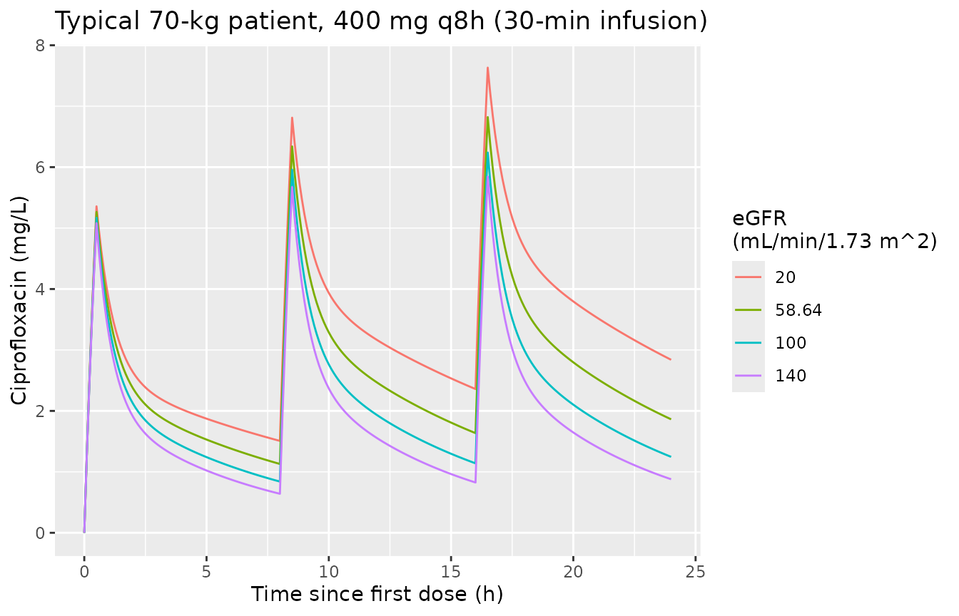
The clearance of the typical patient must equal the printed 14.7 L/h, and the eGFR factor must follow Equation 3 exactly (these are typical-value checks with no random draws, so they are tight):
cl_typ <- sim_typ |>
  group_by(CRCL) |>
  summarise(cl = first(cl), .groups = "drop") |>
  mutate(cl_eq3 = 14.7 * (1 + 0.008 * (CRCL - 58.64)))
knitr::kable(cl_typ, digits = 3, caption = "Typical CL (70 kg) against Equation 3.")| CRCL | cl | cl_eq3 |
|---|---|---|
| 20.00 | 10.156 | 10.156 |
| 58.64 | 14.700 | 14.700 |
| 100.00 | 19.564 | 19.564 |
| 140.00 | 24.268 | 24.268 |
Virtual cohort
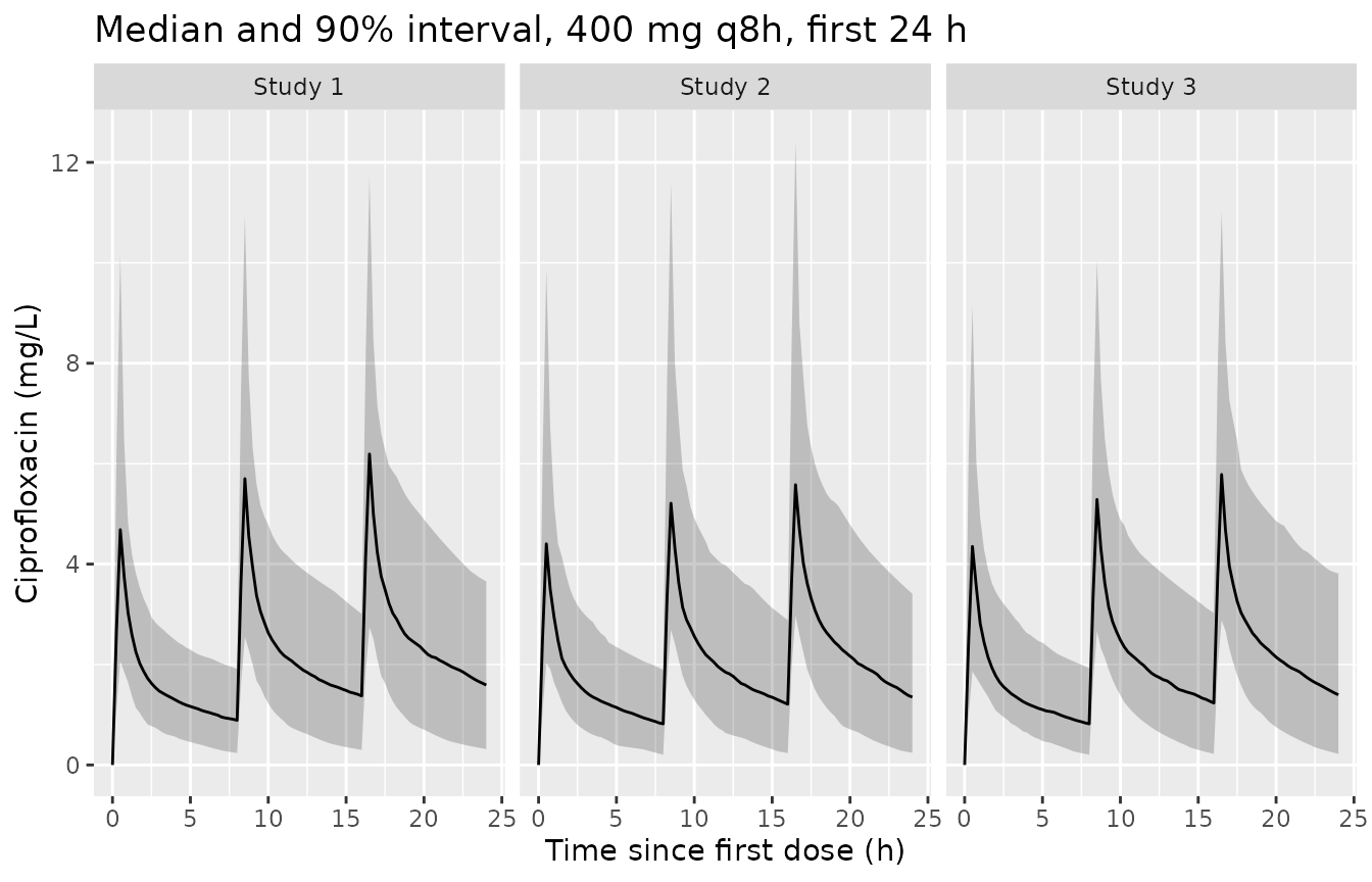
The source data are not public. Each study arm below draws 200 patients whose body weight and eGFR are log-normal with the per-study median and interquartile range of Table 1 (log-scale SD = log(Q3/Q1) / 1.349), truncated to 40-150 kg and 5-200 mL/min/1.73 m^2. The study indicators select each study’s residual error; they have no effect on the PK parameters, so differences in exposure between the simulated arms come only from their covariate distributions.
set.seed(2022)
n_arm <- 200

arms <- tibble::tribble(
  ~study, ~wt_med, ~wt_q1, ~wt_q3, ~gfr_med, ~gfr_q1, ~gfr_q3, ~STUDY_EXPAT, ~STUDY_RDRN,
  "Study 1", 80, 64, 90, 58.5, 31.75, 101.75, 1, 0,
  "Study 2", 80, 66, 98.5, 67, 39, 93, 0, 0,
  "Study 3", 80, 70.75, 93, 56.5, 37.75, 93.75, 0, 1
)

make_arm <- function(a, n, id_offset) {
  tibble(
    id = id_offset + seq_len(n),
    study = a$study,
    WT = pmin(pmax(exp(rnorm(n, log(a$wt_med), log(a$wt_q3 / a$wt_q1) / 1.349)), 40), 150),
    CRCL = pmin(pmax(exp(rnorm(n, log(a$gfr_med), log(a$gfr_q3 / a$gfr_q1) / 1.349)), 5), 200),
    STUDY_EXPAT = a$STUDY_EXPAT,
    STUDY_RDRN = a$STUDY_RDRN
  )
}
subjects <- bind_rows(lapply(seq_len(nrow(arms)), function(i) {
  make_arm(arms[i, ], n_arm, id_offset = (i - 1L) * n_arm)
}))

# 400 mg q8h as a 30-min infusion over the first 24 h (the paper's simulation
# regimen, Methods 2.3.2); the whole window is occasion 1.
events <- bind_rows(
  subjects |> tidyr::crossing(time = c(0, 8, 16)) |>
    mutate(evid = 1L, amt = 400, rate = 800),
  subjects |> tidyr::crossing(time = seq(0, 24, by = 0.25)) |>
    mutate(evid = 0L, amt = 0, rate = 0)
) |>
  mutate(cmt = "central", OCC = 1L) |>
  arrange(id, time, desc(evid))
stopifnot(!anyDuplicated(unique(events[, c("id", "time", "evid")])))

subjects |>
  group_by(study) |>
  summarise(
    n = n(),
    `WT median (kg)` = median(WT),
    `eGFR median` = median(CRCL),
    .groups = "drop"
  ) |>
knitr::kable(digits = 1, caption = "Simulated covariates by study arm.")| study | n | WT median (kg) | eGFR median |
|---|---|---|---|
| Study 1 | 200 | 80.9 | 53.1 |
| Study 2 | 200 | 77.8 | 66.8 |
| Study 3 | 200 | 78.9 | 60.5 |
Simulation
rxode2::rxSetSeed(2022)
sim <- rxode2::rxSolve(mod, events = events, keep = "study") |>
  as.data.frame()
#> ℹ parameter labels from comments will be replaced by 'label()'
#> Warning: some etas defaulted to non-mu referenced, possible parsing error: etaiov_cl_1, etaiov_cl_2, etaiov_cl_3, etaiov_cl_4, etaiov_cl_5, etaiov_cl_6, etaiov_cl_7
#> as a work-around try putting the mu-referenced expression on a simple line
sim |>
  group_by(study, time) |>
  summarise(
    Q05 = quantile(Cc, 0.05), Q50 = median(Cc), Q95 = quantile(Cc, 0.95),
    .groups = "drop"
  ) |>
  ggplot(aes(time, Q50)) +
  geom_ribbon(aes(ymin = Q05, ymax = Q95), alpha = 0.25) +
  geom_line() +
  facet_wrap(~study) +
  labs(
    x = "Time since first dose (h)", y = "Ciprofloxacin (mg/L)",
    title = "Median and 90% interval, 400 mg q8h, first 24 h"
  )
Study-specific residual error
The residual error switches by study. Comparing the simulated
observation (sim) with the individual prediction
(Cc) recovers each study’s error model; the proportional
component is checked on concentrations above 2 mg/L, where study 1’s
additive 0.151 mg/L contributes little.
ruv <- sim |>
  mutate(rel = (sim - Cc) / Cc) |>
  group_by(study) |>
  summarise(
    `SD of (sim - Cc)/Cc, Cc > 2 mg/L` = sd(rel[Cc > 2]),
    `SD of (sim - Cc), Cc < 0.5 mg/L` = sd((sim - Cc)[Cc > 0 & Cc < 0.5]),
    .groups = "drop"
  ) |>
  mutate(`Table 2 proportional` = c(0.175, 0.137, 0.245))
knitr::kable(ruv, digits = 3)| study | SD of (sim - Cc)/Cc, Cc > 2 mg/L | SD of (sim - Cc), Cc < 0.5 mg/L | Table 2 proportional |
|---|---|---|---|
| Study 1 | 0.182 | 0.165 | 0.175 |
| Study 2 | 0.136 | 0.047 | 0.137 |
| Study 3 | 0.241 | 0.082 | 0.245 |
# Proportional SD at high Cc: study 1 additionally carries the additive term
# (0.151 / 2 = 0.076 at the 2 mg/L floor), so it is checked only for being
# at least its proportional SD; studies 2 and 3 are pure proportional.
stopifnot(
  abs(ruv[[2]][2] / 0.137 - 1) < 0.15,
  abs(ruv[[2]][3] / 0.245 - 1) < 0.15,
  ruv[[2]][1] > 0.175 * 0.9
)
Replicate Figure 4: AUC24 and target attainment
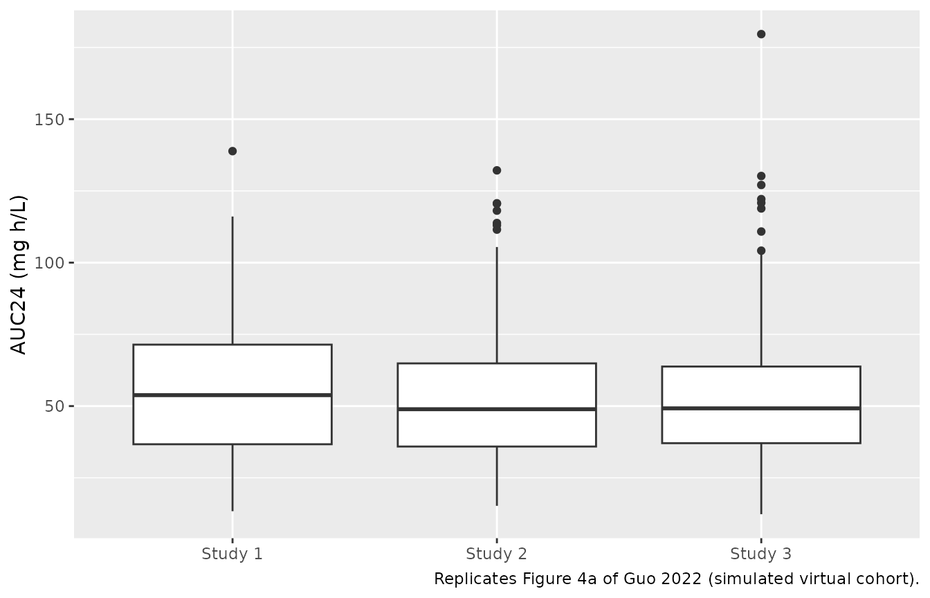
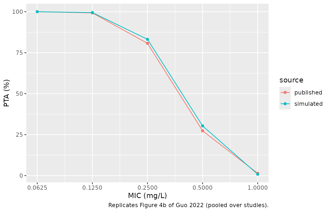
Guo 2022 simulated 400 mg t.i.d. over the first 24 h from posterior samples of each patient’s PK parameters and reported a mean AUC24 of 47.7, 47.6 and 58 mg h/L for studies 1, 2 and 3 (SD 22.8-25.8), and a probability of target attainment (AUC24 / MIC >= 125) at MIC 0.5 mg/L of 21%, 18% and 38%. The packaged model carries no study effect on PK, so the study differences in Figure 4 (which come from the study-specific posterior distributions, Table 3) cannot be reproduced; the comparison below is made against the patient-weighted pooled values (42, 39 and 59 patients).
sim_nca <- sim |>
  filter(!is.na(Cc)) |>
  select(id, time, Cc, study)
conc_obj <- PKNCA::PKNCAconc(sim_nca, Cc ~ time | study + id)

dose_df <- events |>
  filter(evid == 1) |>
  select(id, time, amt, study)
dose_obj <- PKNCA::PKNCAdose(dose_df, amt ~ time | study + id)

intervals <- data.frame(start = 0, end = 24, auclast = TRUE, cmax = TRUE)
nca_res <- PKNCA::pk.nca(PKNCA::PKNCAdata(conc_obj, dose_obj, intervals = intervals))

auc24 <- as.data.frame(nca_res) |>
  filter(PPTESTCD == "auclast") |>
  select(id, study, auc24 = PPORRES)
# Replicates Figure 4a of Guo 2022 (AUC24 box plot by study).
ggplot(auc24, aes(study, auc24)) +
  geom_boxplot() +
  labs(
    x = NULL, y = "AUC24 (mg h/L)",
    caption = "Replicates Figure 4a of Guo 2022 (simulated virtual cohort)."
  )
w <- c(42, 39, 59)
published <- tibble(
  group = "Pooled (patient-weighted)",
  auclast = sum(w * c(47.7, 47.6, 58)) / sum(w)
)
simulated <- tibble(group = "Pooled (patient-weighted)", auclast = mean(auc24$auc24))
cmp <- nlmixr2lib::ncaComparisonTable(
  simulated = simulated,
  reference = published,
  by = "group",
  units = c(auclast = "mg*h/L"),
  tolerance_pct = 20
)
knitr::kable(cmp, caption = "Mean AUC0-24 after 400 mg q8h: simulated vs. Guo 2022 (Results 3.2.2).")| NCA parameter | group | Reference | Simulated | % diff |
|---|---|---|---|---|
| AUClast (mg*h/L) | Pooled (patient-weighted) | 52 | 53.9 | +3.6% |
auc24 |>
  group_by(study) |>
  summarise(mean = mean(auc24), sd = sd(auc24), median = median(auc24), .groups = "drop") |>
  mutate(`published mean` = c(47.7, 47.6, 58)) |>
knitr::kable(digits = 1, caption = "Simulated AUC0-24 (mg h/L) by study arm.")| study | mean | sd | median | published mean |
|---|---|---|---|---|
| Study 1 | 55.0 | 23.6 | 53.8 | 47.7 |
| Study 2 | 53.0 | 23.0 | 48.9 | 47.6 |
| Study 3 | 53.6 | 24.3 | 49.2 | 58.0 |
# Replicates Figure 4b of Guo 2022. Published pooled PTA is the
# patient-weighted mean of the three study curves; the 0.5 mg/L values are
# printed in Results 3.2.2, the others are read from Figure 4b.
mics <- c(0.0625, 0.125, 0.25, 0.5, 1)
pta_pub <- tibble(
  mic = mics,
  s1 = c(100, 99, 73, 21, 1),
  s2 = c(100, 100, 75, 18, 1),
  s3 = c(100, 99, 90, 38, 2)
) |>
  mutate(published = (42 * s1 + 39 * s2 + 59 * s3) / 140)
pta_sim <- tibble(mic = mics) |>
  rowwise() |>
  mutate(simulated = 100 * mean(auc24$auc24 / mic >= 125)) |>
  ungroup()
pta <- left_join(pta_pub |> select(mic, published), pta_sim, by = "mic")
pta |>
  mutate(mic = format(mic)) |>
  dplyr::rename("MIC (mg/L)" = mic, "Published PTA (%)" = published, "Simulated PTA (%)" = simulated) |>
knitr::kable(digits = 1, caption = "Pooled PTA (%), AUC24/MIC >= 125.")| MIC (mg/L) | Published PTA (%) | Simulated PTA (%) |
|---|---|---|
| 0.0625 | 100.0 | 100.0 |
| 0.1250 | 99.3 | 99.5 |
| 0.2500 | 80.7 | 83.2 |
| 0.5000 | 27.3 | 30.3 |
| 1.0000 | 1.4 | 0.8 |
pta |>
  tidyr::pivot_longer(c(published, simulated), names_to = "source", values_to = "PTA") |>
  ggplot(aes(mic, PTA, colour = source)) +
  geom_line() +
  geom_point() +
  scale_x_log10(breaks = mics) +
  labs(
    x = "MIC (mg/L)", y = "PTA (%)",
    caption = "Replicates Figure 4b of Guo 2022 (pooled over studies)."
  )
# Structural gates on the centre of the AUC distribution and on the
# PTA curve at the MICs where it is neither 0% nor 100%. A mis-transcribed
# CL, dose or eGFR slope moves mean AUC24 by tens of percent.
pct_auc <- 100 * (mean(auc24$auc24) / published$auclast - 1)
stopifnot(
  abs(pct_auc) < 20,
  abs(pta$simulated[pta$mic == 0.25] - pta$published[pta$mic == 0.25]) < 15,
  abs(pta$simulated[pta$mic == 0.5] - pta$published[pta$mic == 0.5]) < 15
)
The pooled mean AUC24 of the virtual cohort is within a few percent of the patient-weighted published mean, the per-arm SDs fall in the published 22.8-25.8 mg h/L range, and the pooled PTA curve follows Figure 4b across the MIC range. The higher AUC24 of study 3 in the paper is not reproduced: in the model the three arms differ only by covariates, whereas the paper’s study 3 patients had a lower posterior mean CL (12.6 versus 16.6 and 16 L/h, Table 3) that the covariates do not explain.
Inter-occasion variability
Clearance varies between 24-h occasions with a CV of 13.6%. With seven occasions the within-subject difference of log(CL) between two occasions has an SD of sqrt(2 x 0.01833) = 0.191.
iov_subj <- tibble(id = 1:200, WT = 70, CRCL = 58.64, STUDY_EXPAT = 0, STUDY_RDRN = 0)
iov_events <- iov_subj |>
  tidyr::crossing(OCC = 1:7) |>
  mutate(time = (OCC - 1) * 24 + 12, evid = 0L, amt = 0, cmt = "central")
rxode2::rxSetSeed(7)
sim_iov <- rxode2::rxSolve(mod, events = iov_events) |>
  as.data.frame()
iov_sd <- sim_iov |>
  group_by(id) |>
  summarise(d = log(cl[OCC == 2]) - log(cl[OCC == 1]), .groups = "drop") |>
  summarise(sd = sd(d)) |>
  pull(sd)
iov_sd
#> [1] 0.1894754
stopifnot(abs(iov_sd / sqrt(2 * 0.018327) - 1) < 0.25)
Assumptions and deviations
-
eGFR effect. Equation 3 multiplies CL by
1 + 0.008 x (eGFR - 58.64), i.e. a 0.8% change per mL/min/1.73 m^2. The Results prose describes the same coefficient as an absolute change (“CL increases 0.008 L/h when eGFR increases 1 mL/min/1.73 m^2”), which would be an effect about 15-fold smaller. The printed equation is implemented. -
Number of occasions. The paper defines every 24 h
as an occasion but does not say how many occasions the data spanned.
Seven are encoded (the first week of therapy), each sharing the single
estimated IOV variance. Records with
OCCoutside 1-7 carry no IOV; the paper’s own exposure simulation is restricted to the first 24 h (OCC = 1). -
Study indicators. Study 2 (Radboud UMC, Gieling
2020) is the reference stratum;
STUDY_EXPAT(study 1) andSTUDY_RDRN(study 3) select the other residual-error models and affect nothing else. For a new patient any stratum may be used; the choice only changes the simulated measurement noise. - Study differences in exposure. The between-study differences in Figure 4 and Table 3 come from posterior samples of each patient’s random effects, which are not published. They are not part of the population model and are not reproduced; only the pooled AUC24 and PTA are compared.
- Virtual cohort. Body weight and eGFR are drawn independently as log-normal variables matched to the Table 1 per-study median and IQR; the paper’s simulation instead used the observed patients. The infusion duration of the paper’s simulation is not stated; 30 min is used.
- Figure 4b reading. The PTA values at MICs other than 0.5 mg/L were read from Figure 4b by the maintainers (to about 2 percentage points). The figure caption gives 4200, 5900 and 3900 simulated patients for studies 1, 2 and 3, which does not match 100 samples x 42, 39 and 59 patients; the study 2 and study 3 counts appear swapped.
- Errata. No correction notice was found in Europe PMC as of 2026-10-02.