Apitolisib pAkt-driven translational PK-PD-efficacy (Moein 2024)
Source:vignettes/articles/Moein_2024_apitolisib.Rmd
Moein_2024_apitolisib.RmdModel and source
Moein et al. asked a translational question: having built an integrated PK-PD-efficacy model in xenograft mice, how well does it predict what was later seen in patients? They answered it by building the same three-layer model twice – once on 786-O renal-cell-carcinoma xenografts and once on two phase 1 dose-escalation studies – and comparing the two parameter sets. Both models are packaged here.
mouse_fn <- readModelDb("Moein_2024_apitolisib_mouse")
human_fn <- readModelDb("Moein_2024_apitolisib_human")- Citation: Moein A, Jin JY, Wright MR, Alicke B, Wong H. Retrospective Assessment of Translational Pharmacokinetic-Pharmacodynamic Modeling Performance: A Case Study with Apitolisib, a Dual PI3K/mTOR Inhibitor. Drugs R D. 2024;24(2):155-167. doi:10.1007/s40268-024-00459-5. PMCID PMC11315854. Structural equations from Methods Eqs. 2-5; parameter values from Tables 1 and 3; NONMEM control stream from Supplementary Information Online Resource 2 (part I). Companion human model: modellib(‘Moein_2024_apitolisib_human’).
- Article: https://doi.org/10.1007/s40268-024-00459-5
- PubMed Central (open access): https://www.ncbi.nlm.nih.gov/pmc/articles/PMC11315854/
- Supplementary Information (Online Resource 1, model-development narrative; Online Resource 2, the complete NONMEM control streams for both integrated models): available from the article page above.
The drug is apitolisib (GDC-0980), a dual PI3K/mTOR
inhibitor. The translational biomarker is phosphorylated Akt
(serine 473), expressed throughout as %pAkt – a
percentage of the drug-free control (xenografts) or pre-dose baseline
(patients), so it starts at 100 by construction.
The three layers
Both models are one ODE system stacking three sequentially-fitted layers.
| Layer | Xenograft model | Human model | Source |
|---|---|---|---|
| 1. PK | 1-compartment, first-order oral absorption | 2-compartment, first-order oral absorption + lag | Methods Sects. 2.3.1 / 2.3.2 |
| 2. pAkt | indirect response, drug inhibits kin; pAkt measured in
tumour tissue
|
same structure; pAkt measured in platelet-rich plasma | Methods Eq. 3 |
| 3. Efficacy | exponential tumour volume growth opposed by a sigmoid shrinkage rate | exponential RECIST sum of longest diameters growth, same form | Methods Eqs. 4-5 |
The equations, verbatim from Methods:
Note the coupling: the drug acts on pAkt, and it is the percent
pAkt inhibition I – not the drug concentration – that
drives tumour shrinkage. That is what makes KI50 a
biomarker-axis parameter rather than a concentration (see the Source
trace below).
mouse <- rxode2::rxode2(mouse_fn)
#> ℹ parameter labels from comments will be replaced by 'label()'
human <- rxode2::rxode2(human_fn)
#> ℹ parameter labels from comments will be replaced by 'label()'

data.frame(
  model = c("xenograft (mouse)", "phase 1 (human)"),
  states = c(paste(mouse$state, collapse = ", "),
             paste(human$state, collapse = ", ")),
  n_theta = c(length(mouse$theta), length(human$theta))
) |>
knitr::kable()| model | states | n_theta |
|---|---|---|
| xenograft (mouse) | depot, central, pakt, tumor_vol | 15 |
| phase 1 (human) | depot, central, peripheral1, pakt, tumor_size | 18 |
Population
pop_m <- mouse_fn()$population
pop_h <- human_fn()$population
Xenografts (mouse (female beige nude XID, bg.nu.xid
Harlan; subcutaneous 786-O human renal cell adenocarcinoma xenograft)):
64 mice across 3 studies contributed 381 tumour-volume observations.
Median baseline tumour volume was 173.5 mm^3. Tumour volume was measured
with digital calipers as TV = length * width^2 * 0.5
(Methods Eq. 1). The pAkt sub-study used separate animals, with tumours
collected at 0.5, 2, 6, 12, 18 and 24 h post-dose and pAkt quantified by
Meso Scale Discovery assay in tumour tissue.
Patients: the sub-populations differ by layer. The population PK model used n = 146 patients with 1835 PK observations; the pAkt PK-PD model used the n = 37 patients in whom platelet-rich-plasma pAkt was measured; and the integrated PK-PD-efficacy model used the 117 evaluable patients contributing 417 tumour-size observations (Results Sect. 3.3). Median baseline tumour size (RECIST sum of longest diameters) was 130.0 mm. Both studies (NCT00854152, NCT00854126) were 3+3 dose escalations in advanced solid tumours or non-Hodgkin’s lymphoma. No covariates were retained in any layer of either model.
The full metadata is available programmatically:
data.frame(
  field = c("species", "n_subjects", "n_studies", "disease_state"),
  xenograft = c(pop_m$species, pop_m$n_subjects, pop_m$n_studies,
                pop_m$disease_state),
  human = c(pop_h$species, pop_h$n_subjects, pop_h$n_studies,
            pop_h$disease_state)
) |>
knitr::kable()| field | xenograft | human |
|---|---|---|
| species | mouse (female beige nude XID, bg.nu.xid Harlan; subcutaneous 786-O human renal cell adenocarcinoma xenograft) | human |
| n_subjects | 64 | 117 |
| n_studies | 3 | 2 |
| disease_state | subcutaneous 786-O human renal cell adenocarcinoma (RCC) xenograft | advanced solid tumors or non-Hodgkin’s lymphoma |
Source trace
Every ini() value carries an in-file comment naming its
source location. They are collected here for review.
| Layer | Parameter | Xenograft value | Human value | Source location |
|---|---|---|---|---|
| PK | ka |
1.1 1/h | 3.35 1/h | Results Sects. 3.1.1 / 3.1.2 |
| PK |
cl (CL/F) |
0.387 L/h/kg | 21.3 L/h | Results Sects. 3.1.1 / 3.1.2 |
| PK |
vc (V/F, V1/F) |
1.13 L/kg | 210.6 L | Results Sects. 3.1.1 / 3.1.2 |
| PK |
vp (V2/F) |
n/a (1-cmt) | 639.1 L | Results Sect. 3.1.2 |
| PK |
q (CLd/F) |
n/a (1-cmt) | 5.93 L/h | Results Sect. 3.1.2 |
| PK | tlag |
n/a | 0.465 h | Results Sect. 3.1.2 |
| PK | IIV variances | not reported | 0.17 / 0.0639 / 0.881 / 0.208 / 2.09 | Results Sect. 3.1.2 |
| pAkt | ic50 |
403 ug/L | 9.32 ug/L | Table 1 / Table 2 |
| pAkt | kin |
88,698 %/h | 88,699 %/h | Table 1 / Table 2 |
| pAkt | kout |
886.98 1/h (derived) | 886.99 1/h (derived) | Table 1 / Table 2, footnote kout = kin/%pAkt(0)
|
| pAkt | imax |
1 (fix) | 1 (fix) | Table 1 / Table 2 |
| pAkt |
hill_pakt (gamma1) |
1 (fix) | 1 (fix) | Table 1 / Table 2 |
| pAkt | propSd_pakt |
0.353 | 0.672 | Table 1 / Table 2 |
| pAkt | IIV ic50
|
not estimated | 0.296 | Table 2 |
| Efficacy |
p (Kg) |
0.0057 1/h | 0.0097 1/week | Table 3 / Table 4 |
| Efficacy | kmax |
0.0194 1/h | 0.0142 1/week | Table 3 / Table 4 |
| Efficacy |
ki50 (KI50) |
67.2 %pAkt inhibition | 58.0 %pAkt inhibition | Table 3 / Table 4 |
| Efficacy |
hill_ks (gamma2) |
9.4 | 6.52 | Table 3 / Table 4 |
| Efficacy | propSd_tumor_* |
0.248 | 0.141 | Table 3 / Table 4 |
| Efficacy | IIV p, kmax
|
0.0276, 0.0529 | 0.668, 0.377 | Table 3 / Table 4 |
| Efficacy | IIV ki50, hill_ks
|
not estimated | 0.0225 (fix), 0.0225 (fix) | Table 4 |
| Baseline | rbase_tumor |
173.5 mm^3 (median) | 130.0 mm (median) | Results Sect. 3.3 |
| Equations | Eqs. 2-5 | – | – | Methods Sects. 2.4, 2.5 |
Mixed time units are real, not a transcription
error. Table 3 reports the xenograft Kg and
Kmax per hour; Table 4 reports the patient
values per week. Both packaged models use an hour time
base, so the human file writes log(0.0097 / 168) and
log(0.0142 / 168) – keeping the published number visible at
the assignment. The cross-species fold-differences quoted in Results
only reconcile under this reading, which is checked as a gate below.
Validation
The paper reports no NCA table, so most gates below are exact identities: a quantity the published parameters determine analytically, recomputed from the packaged model. Where the paper does state a number (the 98.7-fold growth-rate ratio, the 43-fold IC50 ratio, the 61%/65% stasis inhibitions, the 0.3 and 0.1 1/h elimination rate constants), the gate compares against that number.
# Pull the packaged values back out so every gate below is computed from the
# model file rather than from numbers retyped into this vignette.
theta <- function(mod, nm) unname(mod$theta[[nm]])

m_cl <- exp(theta(mouse, "lcl")); m_vc <- exp(theta(mouse, "lvc"))
m_ka <- exp(theta(mouse, "lka")); m_ic50 <- exp(theta(mouse, "lic50"))
m_p <- exp(theta(mouse, "lp")); m_kmax <- exp(theta(mouse, "lkmax"))
m_ki50 <- exp(theta(mouse, "lki50")); m_g2 <- exp(theta(mouse, "lhill_ks"))
m_base <- exp(theta(mouse, "lrbase_tumor"))

h_cl <- exp(theta(human, "lcl")); h_vc <- exp(theta(human, "lvc"))
h_vp <- exp(theta(human, "lvp")); h_q <- exp(theta(human, "lq"))
h_ic50 <- exp(theta(human, "lic50"))
h_p <- exp(theta(human, "lp")); h_kmax <- exp(theta(human, "lkmax"))
h_ki50 <- exp(theta(human, "lki50")); h_g2 <- exp(theta(human, "lhill_ks"))
h_base <- exp(theta(human, "lrbase_tumor"))
Layer 1 – PK
Elimination rate constants (Results Sect. 3.1.2)
The paper contrasts “a faster elimination rate constant (CL/V) … in xenografts (0.3 1/h) compared with patients (0.1 1/h)”.
data.frame(
  quantity = c("xenograft CL/V (1/h)", "patient CL/V1 (1/h)"),
  packaged = round(c(m_cl / m_vc, h_cl / h_vc), 3),
  published = c(0.3, 0.1)
) |>
knitr::kable()| quantity | packaged | published |
|---|---|---|
| xenograft CL/V (1/h) | 0.342 | 0.3 |
| patient CL/V1 (1/h) | 0.101 | 0.1 |
Body-weight-normalised patient PK (Results Sect. 3.1.2)
An exact arithmetic check that the packaged absolute values are the ones the paper normalised to 70 kg.
data.frame(
  parameter = c("CL/F", "V1/F", "V2/F", "CLd/F"),
  packaged_per_70kg = round(c(h_cl, h_vc, h_vp, h_q) / 70, 3),
  published_per_kg = c(0.304, 3.01, 9.13, 0.085)
) |>
knitr::kable()| parameter | packaged_per_70kg | published_per_kg |
|---|---|---|
| CL/F | 0.304 | 0.304 |
| V1/F | 3.009 | 3.010 |
| V2/F | 9.130 | 9.130 |
| CLd/F | 0.085 | 0.085 |
NCA of the simulated single-dose PK
Both PK layers are linear, so AUC(0-inf) = Dose / CL is
an exact identity that the NCA must recover. Deterministic
(typical-value) profiles are used so the identity is testable without
Monte-Carlo noise.
# zeroRe() mutates the object it is given, so build the typical-value models
# from fresh readModelDb() calls and never reuse them for stochastic work.
mouse_typ <- rxode2::zeroRe(rxode2::rxode2(readModelDb("Moein_2024_apitolisib_mouse")))
#> ℹ parameter labels from comments will be replaced by 'label()'
human_typ <- rxode2::zeroRe(rxode2::rxode2(readModelDb("Moein_2024_apitolisib_human")))
#> ℹ parameter labels from comments will be replaced by 'label()'

mouse_pk_doses <- c(1, 5, 10)      # mg/kg, Methods Sect. 2.1 PK study
human_pk_doses <- c(10, 50, 200)   # mg, spanning the 2-200 mg phase 1 range

# Dense early grid so Cmax is resolved; long tail so aucinf extrapolation is small.
mouse_grid <- sort(unique(c(seq(0, 4, by = 0.05), seq(4, 48, by = 0.25))))
human_grid <- sort(unique(c(seq(0, 8, by = 0.05), seq(8, 336, by = 1))))

# Both models declare three endpoints (Cc, pakt, tumour), so rxode2 requires
# every observation record to name one. `dvid = 1` selects Cc; the solver
# returns every state and algebraic observable as a column regardless, which is
# what the pAkt and tumour sections below read.
obs_rows <- function(ids, times) {
  expand.grid(id = ids, time = times) |>
    dplyr::mutate(amt = NA_real_, evid = 0L, cmt = NA_character_, dvid = 1L)
}
dose_rows <- function(ids, times, amt, cmt = "depot") {
  expand.grid(id = ids, time = times) |>
    dplyr::mutate(amt = amt, evid = 1L, cmt = cmt, dvid = NA_integer_)
}

build_pk_ev <- function(doses, grid) {
  dplyr::bind_rows(lapply(seq_along(doses), function(i) {
    dplyr::bind_rows(dose_rows(i, 0, doses[i]), obs_rows(i, grid))
  })) |>
    dplyr::mutate(dose_level = doses[id])
}

mouse_pk <- rxode2::rxSolve(
  mouse_typ, build_pk_ev(mouse_pk_doses, mouse_grid),
  omega = NA, returnType = "data.frame", keep = "dose_level"
)
#> Warning: multi-subject simulation without without 'omega'
human_pk <- rxode2::rxSolve(
  human_typ, build_pk_ev(human_pk_doses, human_grid),
  omega = NA, returnType = "data.frame", keep = "dose_level"
)
#> Warning: multi-subject simulation without without 'omega'
run_nca <- function(sim, dose_unit_scale) {
  conc <- sim |>
    dplyr::filter(!is.na(Cc)) |>
    dplyr::mutate(treatment = paste(dose_level, dose_unit_scale)) |>
    dplyr::select(id, time, Cc, treatment)
  # A time-zero record must be present or PKNCA warns once per subject that the
  # AUC interval starts before the first measurement.
  stopifnot(all(tapply(conc$time, conc$id, min) == 0))

  dose_df <- conc |>
    dplyr::group_by(id, treatment) |>
    dplyr::summarise(time = 0, .groups = "drop") |>
    dplyr::mutate(amt = as.numeric(sub(" .*$", "", treatment)))

  o_conc <- PKNCA::PKNCAconc(conc, Cc ~ time | id / treatment)
  o_dose <- PKNCA::PKNCAdose(dose_df, amt ~ time | id)
  intervals <- data.frame(
    start = 0, end = Inf,
    cmax = TRUE, tmax = TRUE, auclast = TRUE,
    aucinf.obs = TRUE, half.life = TRUE
  )
  res <- PKNCA::pk.nca(PKNCA::PKNCAdata(o_conc, o_dose, intervals = intervals))
  as.data.frame(res$result)
}

mouse_nca <- run_nca(mouse_pk, "mg/kg")
human_nca <- run_nca(human_pk, "mg")
The exact identities to hit:
AUC(0-inf) = Dose * 1000 / CL (the * 1000
converts the mg dose to the ug concentration scale), and, for the
one-compartment xenograft model, the closed-form oral Cmax
and Tmax.
m_kel <- m_cl / m_vc
m_tmax <- log(m_ka / m_kel) / (m_ka - m_kel)
m_cmax <- function(d) {
  d / m_vc * 1000 * m_ka / (m_ka - m_kel) *
    (exp(-m_kel * m_tmax) - exp(-m_ka * m_tmax))
}

mouse_ref <- data.frame(
  treatment = paste(mouse_pk_doses, "mg/kg"),
  cmax = m_cmax(mouse_pk_doses),
  tmax = m_tmax,
  aucinf.obs = mouse_pk_doses * 1000 / m_cl,
  half.life = log(2) / m_kel
)

mouse_sim_wide <- mouse_nca |>
  dplyr::filter(PPTESTCD %in% c("cmax", "tmax", "aucinf.obs", "half.life")) |>
  dplyr::select(treatment, PPTESTCD, PPORRES) |>
  tidyr::pivot_wider(names_from = PPTESTCD, values_from = PPORRES)

nlmixr2lib::ncaComparisonTable(
  simulated = mouse_sim_wide,
  reference = mouse_ref,
  by = "treatment",
  params = c("cmax", "tmax", "aucinf.obs", "half.life")
) |>
  knitr::kable(
    caption = paste(
      "Xenograft PK: simulated NCA vs the closed-form one-compartment oral",
      "identities implied by the packaged CL/F, V/F and ka."
    )
)| NCA parameter | treatment | Reference | Simulated | % diff |
|---|---|---|---|---|
| Cmax | 1 mg/kg | 522 | 522 | -0.0% |
| Cmax | 5 mg/kg | 2610 | 2610 | -0.0% |
| Cmax | 10 mg/kg | 5220 | 5220 | -0.0% |
| Tmax | 1 mg/kg | 1.54 | 1.55 | +0.6% |
| Tmax | 5 mg/kg | 1.54 | 1.55 | +0.6% |
| Tmax | 10 mg/kg | 1.54 | 1.55 | +0.6% |
| AUC0-∞ (obs) | 1 mg/kg | 2580 | 2580 | -0.0% |
| AUC0-∞ (obs) | 5 mg/kg | 12900 | 12900 | -0.0% |
| AUC0-∞ (obs) | 10 mg/kg | 25800 | 25800 | -0.0% |
| t½ | 1 mg/kg | 2.02 | 2.04 | +0.7% |
| t½ | 5 mg/kg | 2.02 | 2.04 | +0.7% |
| t½ | 10 mg/kg | 2.02 | 2.04 | +0.7% |
For the two-compartment patient model the terminal half-life is the slower eigenvalue of the disposition matrix.
h_kel <- h_cl / h_vc; h_k12 <- h_q / h_vc; h_k21 <- h_q / h_vp
h_sum <- h_kel + h_k12 + h_k21
h_beta <- 0.5 * (h_sum - sqrt(h_sum^2 - 4 * h_kel * h_k21))

human_ref <- data.frame(
  treatment = paste(human_pk_doses, "mg"),
  aucinf.obs = human_pk_doses * 1000 / h_cl,
  half.life = log(2) / h_beta
)

human_sim_wide <- human_nca |>
  dplyr::filter(PPTESTCD %in% c("aucinf.obs", "half.life")) |>
  dplyr::select(treatment, PPTESTCD, PPORRES) |>
  tidyr::pivot_wider(names_from = PPTESTCD, values_from = PPORRES)

nlmixr2lib::ncaComparisonTable(
  simulated = human_sim_wide,
  reference = human_ref,
  by = "treatment",
  params = c("aucinf.obs", "half.life")
) |>
  knitr::kable(
    caption = paste(
      "Patient PK: simulated NCA vs the exact Dose/CL identity and the",
      "terminal eigenvalue of the packaged two-compartment disposition."
    )
)| NCA parameter | treatment | Reference | Simulated | % diff |
|---|---|---|---|---|
| AUC0-∞ (obs) | 10 mg | 469 | 469 | -0.0% |
| AUC0-∞ (obs) | 50 mg | 2350 | 2350 | -0.0% |
| AUC0-∞ (obs) | 200 mg | 9390 | 9390 | -0.0% |
| t½ | 10 mg | 97.1 | 96.7 | -0.4% |
| t½ | 50 mg | 97.1 | 96.7 | -0.4% |
| t½ | 200 mg | 97.1 | 96.7 | -0.4% |
Layer 2 – pAkt (replicates Figure 1)
Figure 1A shows mean tumour-tissue %pAkt versus time in
786-O xenografts after single oral doses of 0.3, 3 and 10 mg/kg; Figure
1B shows the surrogate-plasma equivalent in patients.
pakt_profile <- function(mod, doses, grid, unit) {
  ev <- dplyr::bind_rows(lapply(seq_along(doses), function(i) {
    dplyr::bind_rows(dose_rows(i, 0, doses[i]), obs_rows(i, grid))
  })) |>
    dplyr::mutate(dose_level = doses[id])
  rxode2::rxSolve(mod, ev, omega = NA, returnType = "data.frame",
                  keep = "dose_level") |>
    dplyr::mutate(label = factor(paste(dose_level, unit), levels = paste(doses, unit)))
}

pakt_grid <- seq(0, 24, by = 0.05)
mouse_pakt <- pakt_profile(mouse_typ, c(0.3, 3, 10), pakt_grid, "mg/kg")
#> Warning: multi-subject simulation without without 'omega'
human_pakt <- pakt_profile(human_typ, c(2, 8, 12, 30, 70), pakt_grid, "mg")
#> Warning: multi-subject simulation without without 'omega'

dplyr::bind_rows(
  mouse_pakt |> dplyr::mutate(panel = "A: xenograft (tumour tissue)"),
  human_pakt |> dplyr::mutate(panel = "B: patient (platelet-rich plasma)")
) |>
  ggplot2::ggplot(ggplot2::aes(time, pakt, colour = label)) +
  ggplot2::geom_line(linewidth = 0.7) +
  ggplot2::facet_wrap(~panel) +
  ggplot2::scale_x_continuous(breaks = seq(0, 24, by = 6)) +
  ggplot2::labs(
    x = "Time after dose (h)", y = "%pAkt (percent of baseline)",
    colour = "Dose",
    title = "Replicates Figure 1 of Moein 2024"
  ) +
  ggplot2::theme_bw()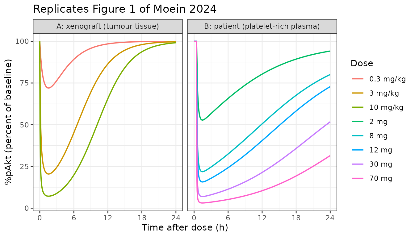
The qualitative features the paper describes are reproduced: a
dose-dependent %pAkt decrease; pronounced suppression by 30
min post-dose in xenografts, sustained for 6-12 h at 3 and 10 mg/kg but
recovering within 1-2 h at 0.3 mg/kg; and, in patients, peak suppression
approaching 90% at doses at or above 12 mg.
nadir <- function(df) {
  df |>
    dplyr::group_by(label) |>
    dplyr::summarise(
      min_pakt = min(pakt),
      max_inhibition_pct = 100 - min(pakt),
      hours_below_50pct = sum(pakt < 50) * 0.05,
      .groups = "drop"
    )
}
dplyr::bind_rows(
  nadir(mouse_pakt) |> dplyr::mutate(model = "xenograft"),
  nadir(human_pakt) |> dplyr::mutate(model = "patient")
) |>
  dplyr::select(model, dplyr::everything()) |>
  dplyr::rename(
    "Model" = model, "Dose" = label, "Nadir %pAkt" = min_pakt,
    "Max inhibition (%)" = max_inhibition_pct,
    "Hours below 50% of baseline" = hours_below_50pct
  ) |>
knitr::kable(digits = 1)| Model | Dose | Nadir %pAkt | Max inhibition (%) | Hours below 50% of baseline |
|---|---|---|---|---|
| xenograft | 0.3 mg/kg | 72.0 | 28.0 | 0.0 |
| xenograft | 3 mg/kg | 20.5 | 79.5 | 6.4 |
| xenograft | 10 mg/kg | 7.2 | 92.8 | 10.1 |
| patient | 2 mg | 52.8 | 47.2 | 0.0 |
| patient | 8 mg | 21.9 | 78.1 | 11.2 |
| patient | 12 mg | 15.7 | 84.3 | 14.7 |
| patient | 30 mg | 6.9 | 93.1 | 22.9 |
| patient | 70 mg | 3.1 | 96.9 | 23.6 |
The indirect-response model collapses to a direct-effect
model, and that is faithful to the published parameters. With
kout = kin/100 = 887 1/h the biomarker pool has a half-life
of 2.8 seconds, so %pAkt tracks the plasma concentration
essentially instantaneously. The gate below compares the ODE solution
against the algebraic quasi-steady-state of Eq. 3,
%pAkt = 100 * (1 - Cc/(IC50 + Cc)). Agreement is near-exact
almost everywhere; the largest deviations are sub-1-percentage-point
excursions confined to the steep post-dose absorption phase, where the
concentration is changing fastest and the pool lags by its 2.8-second
time constant.
direct_effect_dev <- function(sim, ic50) {
  d <- abs(sim$pakt - 100 * (1 - sim$Cc / (ic50 + sim$Cc)))
  c(max = max(d), median = stats::median(d),
    `time of max (h)` = sim$time[which.max(d)])
}
rbind(
  xenograft = direct_effect_dev(mouse_pakt, m_ic50),
  patient = direct_effect_dev(human_pakt, h_ic50)
) |>
  knitr::kable(
    digits = 4,
    caption = paste(
      "Deviation of the ODE solution from the algebraic direct-effect form,",
      "in percentage points of %pAkt."
    )
)| max | median | time of max (h) | |
|---|---|---|---|
| xenograft | 0.5544 | 0.0024 | 0.05 |
| patient | 0.7502 | 0.0025 | 0.50 |
This matters for interpretation: the packaged models carry no
biomarker hysteresis, and kin and kout are
jointly unidentifiable from these data – only their ratio, which fixes
the baseline at 100, has any influence on the solution.
Layer 3 – efficacy (replicates Figure 2)
Figure 2A plots the tumour shrinkage rate constant Ks
against %pAkt inhibition for both species; Figure 2B plots
the same curves normalised to Kmax, which is where the
paper’s “similar shape, different magnitude” conclusion becomes
visible.
ks_curve <- function(I, kmax, ki50, g2) kmax * I^g2 / (ki50^g2 + I^g2)
# Panel A is on a log y-axis, so the grid starts just above zero: Ks is exactly
# 0 at I = 0 and would drop out of a log scale.
I_grid <- seq(0.25, 100, by = 0.25)

# Both curves are put on a per-week basis so panel A is directly comparable
# across species despite Table 3 being per hour and Table 4 per week.
fig2 <- dplyr::bind_rows(
  data.frame(I = I_grid, species = "Xenograft (tumour tissue)",
             ks = ks_curve(I_grid, m_kmax, m_ki50, m_g2) * 168,
             ks_norm = ks_curve(I_grid, m_kmax, m_ki50, m_g2) / m_kmax),
  data.frame(I = I_grid, species = "Typical patient (surrogate plasma)",
             ks = ks_curve(I_grid, h_kmax, h_ki50, h_g2) * 168,
             ks_norm = ks_curve(I_grid, h_kmax, h_ki50, h_g2) / h_kmax)
)

pA <- ggplot2::ggplot(fig2, ggplot2::aes(I, ks, colour = species)) +
  ggplot2::geom_line(linewidth = 0.8) +
  ggplot2::scale_y_log10() +
  ggplot2::labs(x = "%pAkt inhibition", y = "Ks (1/week, log scale)",
                colour = NULL, title = "A: Ks vs %pAkt inhibition") +
  ggplot2::theme_bw() + ggplot2::theme(legend.position = "bottom")

pB <- ggplot2::ggplot(fig2, ggplot2::aes(I, ks_norm, colour = species)) +
  ggplot2::geom_line(linewidth = 0.8) +
  ggplot2::labs(x = "%pAkt inhibition", y = "Ks / Kmax", colour = NULL,
                title = "B: normalised to Kmax") +
  ggplot2::theme_bw() + ggplot2::theme(legend.position = "bottom")

print(pA)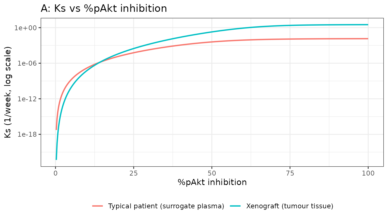
print(pB)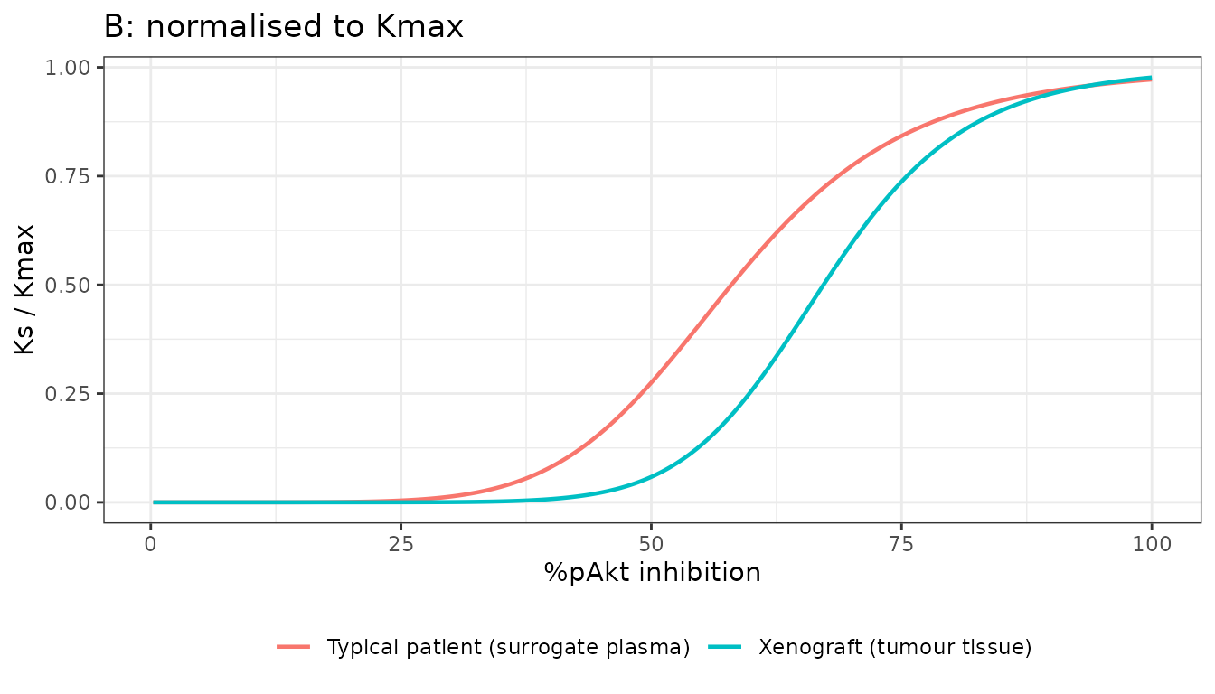
Replicates Figure 2A and 2B of Moein 2024.
The threshold claim: 35-45% pAkt inhibition
The Discussion states that “in both species, a threshold of approximately 35-45% pAkt inhibition is required prior to rapid increases in tumour growth inhibition with increasing pAkt modulation”. The paper read this off Figure 2 by eye rather than defining a numeric criterion, so there is no single value to compare against. What can be checked is that the packaged curves place the onset region in that neighbourhood under any reasonable definition of “onset”. The table sweeps the criterion rather than picking the one that best matches:
inhib_at_frac <- function(frac, ki50, g2) ki50 * (frac / (1 - frac))^(1 / g2)
fracs <- c(0.01, 0.02, 0.05, 0.10, 0.50)
data.frame(
  `Ks as a fraction of Kmax` = paste0(fracs * 100, "%"),
  Xenograft = round(inhib_at_frac(fracs, m_ki50, m_g2), 1),
  `Typical patient` = round(inhib_at_frac(fracs, h_ki50, h_g2), 1),
  check.names = FALSE
) |>
  knitr::kable(
    caption = paste(
      "%pAkt inhibition at which Ks reaches a given fraction of Kmax.",
      "The published onset claim is approximately 35-45%; the 50% row is",
      "KI50 by definition."
    )
)| Ks as a fraction of Kmax | Xenograft | Typical patient |
|---|---|---|
| 1% | 41.2 | 28.7 |
| 2% | 44.4 | 31.9 |
| 5% | 49.1 | 36.9 |
| 10% | 53.2 | 41.4 |
| 50% | 67.2 | 58.0 |
The onset band brackets the published 35-45% claim: the patient curve
crosses it between the 2% and 5% criteria and the xenograft curve
between the 1% and 2% criteria. The two species reach KI50
at 67.2% and 58.0% – the paper’s “similar shape, different magnitude”
observation.
Tumour stasis: the paper’s headline result
Ks = Kg defines stasis, which inverts to
I = KI50 * (Kg / (Kmax - Kg))^(1/gamma2). The paper reports
61% for xenografts and 65% for patients.
stasis_I <- function(p, kmax, ki50, g2) ki50 * (p / (kmax - p))^(1 / g2)
I_stasis_m <- stasis_I(m_p, m_kmax, m_ki50, m_g2)
I_stasis_h <- stasis_I(h_p, h_kmax, h_ki50, h_g2)

data.frame(
  species = c("Xenograft (786-O)", "Typical patient"),
  packaged_stasis_inhibition_pct = round(c(I_stasis_m, I_stasis_h), 2),
  published = c(61, 65)
) |>
knitr::kable()| species | packaged_stasis_inhibition_pct | published |
|---|---|---|
| Xenograft (786-O) | 61.21 | 61 |
| Typical patient | 65.25 | 65 |
Kmax > Kg in both species, which is the paper’s
stated basis for expecting frank regression at sufficient exposure:
data.frame(
  species = c("Xenograft", "Patient"),
  Kg_per_week = round(c(m_p, h_p) * 168, 4),
  Kmax_per_week = round(c(m_kmax, h_kmax) * 168, 4),
  Kmax_exceeds_Kg = c(m_kmax > m_p, h_kmax > h_p)
) |>
knitr::kable()| species | Kg_per_week | Kmax_per_week | Kmax_exceeds_Kg |
|---|---|---|---|
| Xenograft | 0.9576 | 3.2592 | TRUE |
| Patient | 0.0097 | 0.0142 | TRUE |
End-to-end ODE gate: does the stasis concentration actually hold the tumour flat?
The two checks above are algebraic. This one drives the whole packaged ODE system – PK into pAkt into tumour – with a constant infusion set to the plasma concentration that produces exactly the stasis inhibition, and asks whether tumour size is unchanged over a long horizon. It is the strongest available end-to-end test of the coupled model.
# Direct-effect inversion (justified by the gate in Layer 2):
#   I = 100 * Cc / (ic50 + Cc)  =>  Cc = ic50 * I / (100 - I)
css_for <- function(ic50, I) ic50 * I / (100 - I)
# Infusion rate holding that Css: rate = CL * Css, with a /1000 to go from the
# ug/L concentration scale back to the mg dosing scale.
m_css <- css_for(m_ic50, I_stasis_m); m_rate <- m_cl * m_css / 1000
h_css <- css_for(h_ic50, I_stasis_h); h_rate <- h_cl * h_css / 1000

stasis_run <- function(mod, rate, tmax, state) {
  ev <- dplyr::bind_rows(
    dose_rows(1, 0, rate * tmax, cmt = "central") |>
      dplyr::mutate(rate = rate),
    obs_rows(1, c(0, tmax / 2, tmax)) |> dplyr::mutate(rate = NA_real_)
  )
  s <- rxode2::rxSolve(mod, ev, omega = NA, returnType = "data.frame")
  s[[state]][!duplicated(s$time)]
}

m_stasis <- stasis_run(mouse_typ, m_rate, 2000, "tumor_vol")
h_stasis <- stasis_run(human_typ, h_rate, 168 * 40, "tumor_size")

data.frame(
  species = c("Xenograft", "Patient"),
  infusion_conc_ug_L = round(c(m_css, h_css), 2),
  baseline = c(m_base, h_base),
  at_mid_horizon = c(m_stasis[2], h_stasis[2]),
  at_end_horizon = c(m_stasis[3], h_stasis[3]),
  pct_drift_mid_to_end = round(
    100 * (c(m_stasis[3], h_stasis[3]) / c(m_stasis[2], h_stasis[2]) - 1), 6
  )
) |>
knitr::kable(digits = 4)| species | infusion_conc_ug_L | baseline | at_mid_horizon | at_end_horizon | pct_drift_mid_to_end |
|---|---|---|---|---|---|
| Xenograft | 636.05 | 173.5 | 178.9420 | 178.9420 | 0 |
| Patient | 17.50 | 130.0 | 130.2769 | 130.2769 | 0 |
The stasis criterion is the drift between the mid and end of the horizon, which is zero to six decimal places in both species: once the infusion has equilibrated, tumour size is exactly flat over the following 1000 hours (xenograft) and 20 weeks (patient). The small offset from baseline is the growth accrued while the infusion was still approaching steady state – an artefact of starting the infusion at time zero rather than pre-equilibrating, not a failure of the gate.
Drug-free growth must be exactly exponential
With no dose, Eq. 4 reduces to d(Tumor)/dt = Kg * Tumor,
so the solution must equal baseline * exp(Kg * t).
growth_err <- function(mod, state, base, p_val, tmax) {
  ev <- obs_rows(1, seq(0, tmax, length.out = 25))
  s <- rxode2::rxSolve(mod, ev, omega = NA, returnType = "data.frame")
  max(abs(s[[state]] - base * exp(p_val * s$time)))
}
data.frame(
  species = c("Xenograft (0-408 h)", "Patient (0-20 weeks)"),
  max_abs_error = c(
    growth_err(mouse_typ, "tumor_vol", m_base, m_p, 408),
    growth_err(human_typ, "tumor_size", h_base, h_p, 168 * 20)
  )
) |>
knitr::kable()| species | max_abs_error |
|---|---|
| Xenograft (0-408 h) | 0.0011016 |
| Patient (0-20 weeks) | 0.0000176 |
Cross-species translation (the paper’s actual research question)
Every fold-difference quoted in Results Sect. 3.3, recomputed from the two packaged model files. These simultaneously validate the mixed-time-units reading: they only reconcile when Table 3 is per hour and Table 4 is per week.
data.frame(
  quantity = c("Kg fold (xenograft / patient)",
               "Kmax fold (xenograft / patient)",
               "IC50 fold (tumour tissue / surrogate plasma)",
               "KI50 ratio", "gamma2 ratio",
               "Stasis inhibition difference (percentage points)"),
  packaged = round(c(m_p / h_p, m_kmax / h_kmax, m_ic50 / h_ic50,
                     m_ki50 / h_ki50, m_g2 / h_g2,
                     I_stasis_h - I_stasis_m), 2),
  published = c("98.7-fold", "more than 200-fold", "43-fold",
                "\"similar\"", "\"similar\"", "65% vs 61%")
) |>
knitr::kable()| quantity | packaged | published |
|---|---|---|
| Kg fold (xenograft / patient) | 98.72 | 98.7-fold |
| Kmax fold (xenograft / patient) | 229.52 | more than 200-fold |
| IC50 fold (tumour tissue / surrogate plasma) | 43.24 | 43-fold |
| KI50 ratio | 1.16 | “similar” |
| gamma2 ratio | 1.44 | “similar” |
| Stasis inhibition difference (percentage points) | 4.04 | 65% vs 61% |
Virtual cohort and tumour time courses
A stochastic simulation exercising the IIV terms the paper estimated. Cohorts are 100 subjects per dose arm.
set.seed(20240815)
n_per_arm <- 100L

# Rebuild from readModelDb() so the zeroRe()'d objects above are not reused.
human_iiv <- rxode2::rxode2(readModelDb("Moein_2024_apitolisib_human"))
#> ℹ parameter labels from comments will be replaced by 'label()'

human_arms <- c(8, 30, 70)  # mg once daily
obs_times <- seq(0, 168 * 24, by = 168)   # weekly for 24 weeks

human_cohort <- dplyr::bind_rows(lapply(seq_along(human_arms), function(a) {
  # id_offset keeps subject IDs disjoint across arms; duplicate IDs would
  # silently collapse the arms into single (wrong) subjects.
  ids <- (a - 1L) * n_per_arm + seq_len(n_per_arm)
  dplyr::bind_rows(
    dose_rows(ids, seq(0, 168 * 24 - 24, by = 24), human_arms[a]),
    obs_rows(ids, obs_times)
  ) |>
    dplyr::mutate(arm = paste(human_arms[a], "mg QD"))
}))

human_sim <- rxode2::rxSolve(
  human_iiv, human_cohort, omega = human_iiv$omega,
  returnType = "data.frame", keep = "arm"
)

human_sim |>
  dplyr::group_by(arm, time) |>
  dplyr::summarise(
    median = stats::median(tumor_size),
    lo = stats::quantile(tumor_size, 0.05),
    hi = stats::quantile(tumor_size, 0.95),
    .groups = "drop"
  ) |>
  ggplot2::ggplot(ggplot2::aes(time / 168, median, colour = arm, fill = arm)) +
  ggplot2::geom_ribbon(ggplot2::aes(ymin = lo, ymax = hi), alpha = 0.15,
                       colour = NA) +
  ggplot2::geom_line(linewidth = 0.8) +
  ggplot2::geom_hline(yintercept = h_base, linetype = "dashed",
                      colour = "grey40") +
  ggplot2::labs(
    x = "Time (weeks)", y = "Tumour size, RECIST SLD (mm)",
    colour = NULL, fill = NULL,
    title = "Simulated patient tumour size, median with 90% interval",
    subtitle = "Dashed line is the 130 mm median baseline"
  ) +
  ggplot2::theme_bw()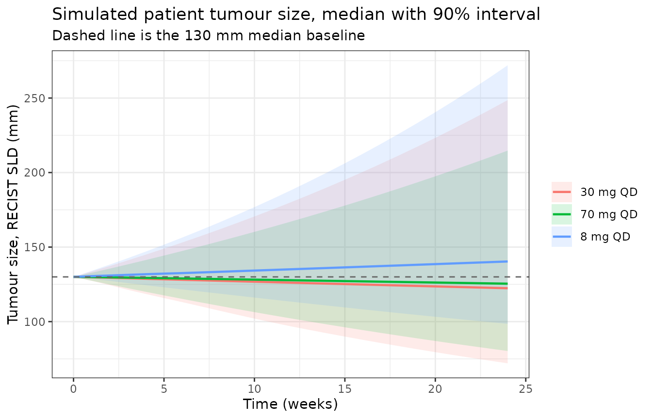
The corresponding xenograft simulation over the 17-day dosing period of the efficacy study:
mouse_iiv <- rxode2::rxode2(readModelDb("Moein_2024_apitolisib_mouse"))
#> ℹ parameter labels from comments will be replaced by 'label()'
mouse_arms <- c(0.256, 2.5, 10)   # mg/kg QD, from the 0.008-11 mg/kg range

mouse_cohort <- dplyr::bind_rows(lapply(seq_along(mouse_arms), function(a) {
  ids <- (a - 1L) * n_per_arm + seq_len(n_per_arm)
  dplyr::bind_rows(
    dose_rows(ids, seq(0, 24 * 16, by = 24), mouse_arms[a]),
    obs_rows(ids, c(0, 72, 96, 168, 240, 264, 336, 408))
  ) |>
    dplyr::mutate(arm = paste(mouse_arms[a], "mg/kg QD"))
}))

mouse_sim <- rxode2::rxSolve(
  mouse_iiv, mouse_cohort, omega = mouse_iiv$omega,
  returnType = "data.frame", keep = "arm"
)

mouse_sim |>
  dplyr::group_by(arm, time) |>
  dplyr::summarise(
    median = stats::median(tumor_vol),
    lo = stats::quantile(tumor_vol, 0.05),
    hi = stats::quantile(tumor_vol, 0.95),
    .groups = "drop"
  ) |>
  ggplot2::ggplot(ggplot2::aes(time / 24, median, colour = arm, fill = arm)) +
  ggplot2::geom_ribbon(ggplot2::aes(ymin = lo, ymax = hi), alpha = 0.15,
                       colour = NA) +
  ggplot2::geom_line(linewidth = 0.8) +
  ggplot2::geom_hline(yintercept = m_base, linetype = "dashed",
                      colour = "grey40") +
  ggplot2::labs(
    x = "Time (days)", y = "Tumour volume (mm^3)", colour = NULL, fill = NULL,
    title = "Simulated 786-O xenograft tumour volume, median with 90% interval",
    subtitle = "Dashed line is the 173.5 mm^3 median baseline"
  ) +
  ggplot2::theme_bw()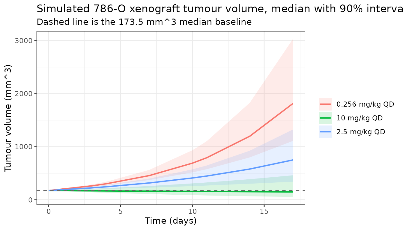
Assumptions and deviations
-
Residual error on plasma apitolisib is not
reported. Methods Sect. 2.3.2 states only that “the residual
error model was a proportional error model”, and the mouse PK results
are reported as “data not shown”. No magnitude appears in the paper,
either table, or either Online Resource. Both files encode
propSd <- fixed(0)per the unreported-RUV convention, so PK simulations are IPRED-scale. The pAkt and tumour residual errors are reported (Tables 1-4) and are encoded. -
Time base. Online Resource 2 part II works in weeks
and rescales the PK by
- Both packaged models use an hour base instead, which keeps every PK
and pAkt value verbatim as published; only the two human tumour rate
constants need conversion, written as
log(0.0097 / 168)andlog(0.0142 / 168)so the published number stays visible at the assignment.
- Both packaged models use an hour base instead, which keeps every PK
and pAkt value verbatim as published; only the two human tumour rate
constants need conversion, written as
-
A transcription slip in the clinical control
stream. Online Resource 2 part II writes
V1 = IV2,V2 = IV3andCP = A(2)/V2.IV3is never declared –$INPUTdeclaresIV1andIV2– and the micro-constants in the same block (S2 = V1,K20 = CL/V1,K23 = Q/V1,K32 = Q/V2), together with Methods Sect. 2.3.2, are consistent with exactly one reading:V1is central,V2is peripheral, andCP = A(central)/V1. The packaged model encodes that standard form. -
The indirect-response layer is numerically a direct-effect
layer. Because
kout = kin/100 = 887 1/h, the pAkt pool equilibrates in seconds and%pAktis very nearly an instantaneous function of plasma concentration (gate above: median deviation from the algebraic direct-effect form far below 0.01 percentage points, with sub-1-percentage-point excursions confined to the steep post-dose absorption phase). This is a property of the published estimates, faithfully reproduced, not an encoding choice. It means the packaged models carry no meaningful biomarker hysteresis, andkin/koutare jointly unidentifiable from these data – only their ratio matters. -
Baseline tumour size is fixed at the reported median, not
estimated. Both control streams read each subject’s own
observed baseline in from the data (
A_0 = TBSL) and Results Sect. 3.3 confirms “individual baseline tumour data were used for model development”. The packaged files setrbase_tumorto the reported median (173.5 mm^3 / 130.0 mm) as a usable simulation default; override it per subject with atumor_vol/tumor_sizeinitial-condition event to reproduce the authors’ setup. - Patient IC50 is carried at the typical value. In the published integrated fit, patients with pAkt data used their individual IC50 and patients without used the typical value (Methods Sect. 2.5). The packaged model applies the typical value with its reported IIV (variance 0.296) to everyone, which is the latter branch. Individual IC50 means by tumour type are in Supplementary Table S1 if a user wants to reproduce the former.
-
PK and IC50 IIV are
fixed(). They were estimated in the separate upstream PK and PK-PD fits and carried into the integrated model, not re-estimated there; only the four tumour IIV terms (etalp,etalkmax,etalki50,etalhill_ks) belonged to the integrated fit.etalki50andetalhill_kswere themselves held at 0.0225 by the authors “to enhance the numerical estimation capability” (Online Resource 1 Sect. II). - No IIV correlations are reported in any layer, so none are encoded.
-
No covariates were retained in any layer of either
model, so
covariateDatais empty in both files. - No published NCA table exists for this paper, so the NCA sections above compare against exact analytic identities implied by the packaged parameters rather than against published Cmax / AUC values. The published quantities that are checked directly are the two elimination rate constants, the 70 kg-normalised PK parameters, the three cross-species fold-differences, and the 61% / 65% stasis inhibitions.
-
Two new canonical names were registered with this
extraction: the
paktcompartment (inst/references/compartment-names.md) and theki50/lki50parameter (inst/references/parameter-names.md).ki50is deliberately distinct fromic50/ec50/kc50because its axis is percent biomarker inhibition, not a drug concentration – both appear in these very files, on different steps of the same cascade. The tumour growth-rate constant the paper callsKgis encoded under the register’s existing generic TGI namep.