Enfortumab vedotin and brentuximab vedotin MMAE drug-drug interactions (Choules 2024)

Model and source

Choules 2024 built a Simcyp antibody-drug conjugate (ADC) module physiologically based pharmacokinetic (PBPK) model for enfortumab vedotin and its released payload monomethyl auristatin E (MMAE), plus a matching model for brentuximab vedotin that shares the same valine-citrulline-MMAE linker and the same MMAE compound file. The brentuximab vedotin model exists in the paper to verify the MMAE drug-drug interaction (DDI) predictions against an observed clinical interaction study, because no dedicated enfortumab vedotin DDI study was run.

Two model files come out of the paper, one per ADC:

• Choules_2024_enfortumab

• Choules_2024_brentuximab

• Citation: Choules MP, Zuo P, Otsuka Y, Garg A, Tang M, Bonate P. Physiologically based pharmacokinetic model to predict drug-drug interactions with the antibody-drug conjugate enfortumab vedotin. J Pharmacokinet Pharmacodyn. 2024;51(5):417-428. doi:10.1007/s10928-023-09877-5. PMID 37624557; PMCID PMC11576838.

• Article: https://doi.org/10.1007/s10928-023-09877-5

• Supplement: https://doi.org/10.1007/s10928-023-09877-5 (Supplementary Information, Tables S1-S5 and Figure S1)

mod_ev <- readModelDb("Choules_2024_enfortumab")
mod_bv <- readModelDb("Choules_2024_brentuximab")

Population

The enfortumab vedotin simulations used the Simcyp cancer population with the plasma tissue-volume scaling factor changed from 1.2 to 1.0, which the authors introduced because the unmodified population under-predicted conjugated antibody Cmax. Single-dose virtual trials were 10 trials of 10 participants; the multiple-dose verification trial was 10 trials of 15 participants (Supplementary Methods). Ages were 24-83 years (26% women) for the 1.25 mg/kg trial, 48-81 years (37% women) for 1.0 mg/kg, 40-90 years (29% women) for the multiple-dose verification trial, and 40-90 years (30% women) for the drug-interaction trials (Table S2).

Choules 2024 Table S4 compares the simulated virtual population against the observed phase 1 EV-101 (NCT02091999) cohort, mean (SD): age 64.9 (12.2) versus 65.1 (10.1) years; weight 72.0 (14.1) versus 80.3 (20.1) kg; plasma albumin 38.2 (7.1) versus 37.5 (4.1) as printed; baseline haematocrit 37.6 (4.65) versus 35.3 (4.76)%. The 72.0 kg simulated mean weight is the reference individual for both model files, and it is the weight used throughout this vignette.

The brentuximab vedotin virtual trials were 10 trials of 12 participants, ages 22-70 years and 40% women, both of which the source states were assumed. No weight is printed for that population; see the Assumptions section.

The same information is available programmatically via each model’s population metadata (readModelDb("Choules_2024_enfortumab")()$population).

Why these files are a compartmental reduction, not a PBPK model

The published model is a Simcyp platform PBPK model. Its whole-body physiology – per-organ volumes and blood flows, tissue:plasma partition coefficients, endosomal volumes and FcRn concentrations for the ADC module, per-enzyme abundances – is a platform database output and is not tabulated anywhere in the paper or its supplement. Reconstructing the model as published is therefore not possible from the source alone.

What the paper does publish is enough to determine a compartmental reduction:

1. The complete MMAE disposition layer. Choules 2024 Table 2 prints the apparent total systemic clearance after intravenous dosing (CL_iv = 2.72 L/h) and the steady-state volume of distribution (Vss = 3.03 L/kg) that the Simcyp retrograde calculation was anchored to. Those two values are used here exactly as printed; nothing about the MMAE layer is fitted.
2. The payload stoichiometry. Table 1 (enfortumab vedotin) and Table S1 (brentuximab vedotin) print the mean drug-antibody ratio and the antibody molecular weight, and Table 2 prints the MMAE molecular weight. Both F_rel (deconjugation) and F_rel (catabolic) are 1, so the mass of MMAE released per unit mass of eliminated antibody is purely stoichiometric.
3. Simulated summary statistics for four dose levels across two ADCs. Tables 3, 6 and S3 print the simulated mean and geometric-mean Cmax, AUC and terminal half-life at enfortumab vedotin 1.0 and 1.25 mg/kg and brentuximab vedotin 1.8 and 2.7 mg/kg.

The four conjugated-antibody parameters per ADC (CL, V1, Q, V2) were determined from item 3 – the published simulated Cmax at both dose levels, the published AUC at both dose levels, the published mean terminal half-life, and the published MMAE Cmax. Because the model is linear and dose-proportional, the two dose levels are one constraint each on the same parameter set rather than two independent fits. The plotted simulated curves in Figures 3, 4 and S1 are arithmetic means, so the arithmetic-mean column of each table is the calibration target.

Everything else the paper publishes was held back and is used below as a zero-free-parameter validation gate: the MMAE AUC, the MMAE half-life, the multiple-dose accumulation table, and the DDI Cmax geometric mean ratios.

Because the artifact is a compartmental model rather than a PBPK model, the file names carry no _pbpk suffix.

Source trace

Equation / parameter	Value	Source location
lcl_mmae (MMAE CL)	2.72 L/h	Table 2, CL_int CYP3A4 source column: “Simcyp retrograde calculated based on apparent CL_iv: 2.72 L/h”
lvc_mmae (MMAE Vss)	3.03 L/kg x 72.0 kg = 218.2 L	Table 2 V_ss; weight from Table S4
mw_mmae	717.98 Da	Table 2, molecular weight
dar (enfortumab vedotin)	3.735	Table 1, mean of the discrete DAR distribution
mw (enfortumab vedotin)	146,664.1 Da	Table 1, molecular weight
dar (brentuximab vedotin)	4.026	Table S1, mean of the discrete DAR distribution
mw (brentuximab vedotin)	148,081 Da	Table S1, molecular weight
Released fraction = 1	1	Table 1 / Table S1, F_rel (deconjugation) = 1 and F_rel (catabolic) = 1
lcl, lvc, lq, lvp (enfortumab vedotin)	0.10969 L/h, 3.4842 L, 0.040504 L/h, 1.6225 L	Derived from Table 3 simulated means (Cmax 25.3 / 20.6 ug/mL; AUC d0-7 32.6 / 26.0 ug*day/mL; t1/2 1.96 day) and the MMAE Cmax 3.52 ng/mL; Figure 3 curve shape
lcl, lvc, lq, lvp (brentuximab vedotin)	0.065773 L/h, 4.0966 L, 0.0057794 L/h, 1.0127 L	Derived from Table S3 simulated means (Cmax 31.5 / 47.2 ug/mL; AUC inf 82.2 / 123 ug*day/mL; t1/2 5.71 day) and the MMAE Cmax 4.62 / 6.96 ng/mL
e_keto_cl_mmae	1 / 1.38 = 0.72464 (EV); 1 / 1.37 = 0.72993 (BV)	Table 5, predicted MMAE AUC ratio with ketoconazole
e_rif_cl_mmae	1 / 0.47 = 2.12766 (both)	Table 5, predicted MMAE AUC ratio with rifampin
ADC 2-compartment disposition; payload released on ADC elimination	n/a	Figure 2 schematic (Simcyp ADC module linked to the small-molecule PBPK model); Methods, “The source of unconjugated MMAE in the model was through catabolism, additional nonspecific plasma clearance, and deconjugation”
Infusion duration 30 min	0.5 h	Methods and Table S2
propSd, propSd_mmae	not reported	Choules 2024 reports no residual-error model; see Errata

Simulation setup

Both models are deterministic: the source is a PBPK simulation study with no population-PK random-effects structure, so the model files carry no eta terms and no residual error. One subject per arm therefore reproduces the model exactly, and no virtual cohort is required.

BW <- 72.0                       # kg, Choules 2024 Table S4 simulated mean weight
INF_DUR <- 0.5                   # h, 30-minute intravenous infusion

# Dense early grid to resolve the end-of-infusion peak, coarser later.
obs_grid <- function(tmax_h) {
  sort(unique(c(
    seq(0, 2, by = 0.05),
    seq(2.5, 48, by = 0.5),
    seq(49, tmax_h, by = 1)
  )))
}

make_arm <- function(id, dose_mgkg, dose_times_h, tmax_h, treatment,
                     keto = 0, rif = 0) {
  tt <- obs_grid(tmax_h)
  amt <- dose_mgkg * BW
  # Both model outputs (Cc, Cc_mmae) are algebraic observables rather than ODE
  # states, so observation rows carry dvid = 1 with cmt = NA. rxode2 returns
  # every algebraic observable as a column on each output row, so one dvid is
  # enough to get both analytes.
  dosing <- data.frame(
    id = id, time = dose_times_h, amt = amt, rate = amt / INF_DUR,
    evid = 1L, cmt = "central", dvid = NA_integer_
  )
  obs <- data.frame(
    id = id, time = tt, amt = NA_real_, rate = NA_real_,
    evid = 0L, cmt = NA_character_, dvid = 1L
  )
  out <- dplyr::bind_rows(dosing, obs)
  out$treatment <- treatment
  out$dose_mgkg <- dose_mgkg
  out$CONMED_KETOCONAZOLE <- keto
  out$CONMED_RIF <- rif
  dplyr::arrange(out, id, time, dplyr::desc(evid))
}

Cc is the conjugated-antibody concentration in ug/mL. The model carries MMAE in the same mg/L system, so Cc_mmae is multiplied by 1000 to reach the ng/mL scale the paper uses.

solve_arms <- function(mod, events) {
  rxode2::rxSolve(
    mod, events = events,
    keep = c("treatment", "dose_mgkg"),
    atol = 1e-10, rtol = 1e-8, returnType = "data.frame"
  ) |>
    dplyr::mutate(Cc_mmae_ng = Cc_mmae * 1000)
}

Enfortumab vedotin: single dose (replicates Figure 3)

ev_single <- dplyr::bind_rows(
  make_arm(1L, 1.25, 0, 168, "1.25 mg/kg"),
  make_arm(2L, 1.00, 0, 168, "1.0 mg/kg")
)
stopifnot(!anyDuplicated(ev_single[, c("id", "time", "evid")]))

sim_ev <- solve_arms(mod_ev, ev_single)
#> Warning: multi-subject simulation without without 'omega'

# Replicates Figure 3a of Choules 2024: simulated semilog conjugated
# enfortumab vedotin concentration after a single 30-minute IV infusion.
sim_ev |>
  dplyr::filter(time > 0) |>
  ggplot(aes(time / 24, Cc, colour = treatment)) +
  geom_line(linewidth = 0.8) +
  scale_y_log10(limits = c(0.1, 100)) +
  labs(x = "Days", y = "Conjugated antibody concentration (ug/mL)",
       colour = NULL,
       title = "Figure 3a - conjugated enfortumab vedotin",
       caption = "Replicates Figure 3a of Choules 2024.")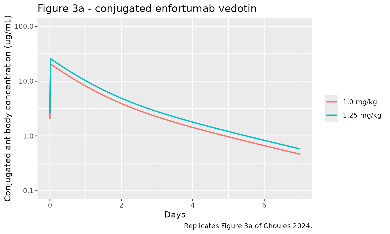

# Replicates Figure 3b of Choules 2024: simulated semilog free MMAE.
sim_ev |>
  dplyr::filter(time > 0) |>
  ggplot(aes(time / 24, Cc_mmae_ng, colour = treatment)) +
  geom_line(linewidth = 0.8) +
  scale_y_log10(limits = c(0.1, 10)) +
  labs(x = "Days", y = "Free MMAE concentration (ng/mL)",
       colour = NULL,
       title = "Figure 3b - free MMAE after enfortumab vedotin",
       caption = "Replicates Figure 3b of Choules 2024.")
#> Warning: Removed 28 rows containing missing values or values outside the scale range
#> (`geom_line()`).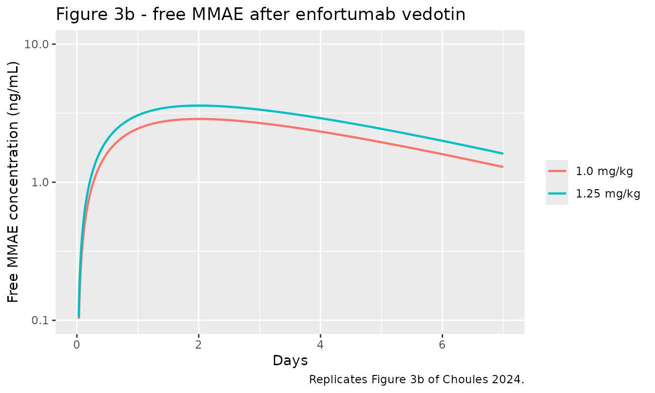

PKNCA validation against Table 3

Choules 2024 Table 3 reports AUC from time 0 to day 7, Cmax and terminal half-life for both analytes. The NCA below uses the same 0-168 h window.

run_nca <- function(sim, events, conc_col, interval) {
  nca_conc <- sim |>
    dplyr::filter(!is.na(.data[[conc_col]])) |>
    dplyr::transmute(id, time, conc = .data[[conc_col]], treatment)
  nca_conc <- dplyr::bind_rows(
    nca_conc,
    nca_conc |> dplyr::distinct(id, treatment) |>
      dplyr::mutate(time = 0, conc = 0)
  ) |>
    dplyr::distinct(id, treatment, time, .keep_all = TRUE) |>
    dplyr::arrange(id, treatment, time)

  nca_dose <- events |>
    dplyr::filter(evid == 1) |>
    dplyr::select(id, time, amt, treatment)

  PKNCA::pk.nca(PKNCA::PKNCAdata(
    PKNCA::PKNCAconc(nca_conc, conc ~ time | treatment + id),
    PKNCA::PKNCAdose(nca_dose, amt ~ time | treatment + id),
    intervals = interval
  ))
}

iv_interval <- function(end, auc = "auclast") {
  out <- data.frame(start = 0, end = end, cmax = TRUE, tmax = TRUE,
                    half.life = TRUE)
  out[[auc]] <- TRUE
  out
}

nca_ev_adc <- run_nca(sim_ev, ev_single, "Cc", iv_interval(168))

# Choules 2024 Table 3, simulated arithmetic means. AUC converted from
# ug*day/mL to ug*h/mL and half-life from days to hours.
ref_ev_adc <- data.frame(
  treatment = c("1.25 mg/kg", "1.0 mg/kg"),
  cmax      = c(25.3, 20.6),
  auclast   = c(32.6, 26.0) * 24,
  half.life = c(1.96, 1.94) * 24
)

tbl_ev_adc <- nlmixr2lib::ncaComparisonTable(
  nca_ev_adc, ref_ev_adc, by = "treatment",
  params = c("cmax", "auclast", "half.life"),
  units = c(cmax = "ug/mL", auclast = "ug*h/mL", half.life = "h")
)
knitr::kable(tbl_ev_adc,
             caption = "Conjugated enfortumab vedotin: simulated vs Choules 2024 Table 3 (simulated mean).")

Conjugated enfortumab vedotin: simulated vs Choules 2024 Table 3 (simulated mean).

NCA parameter	treatment	Reference	Simulated	% diff
Cmax (ug/mL)	1.25 mg/kg	25.3	25.6	+1.0%
Cmax (ug/mL)	1.0 mg/kg	20.6	20.4	-0.8%
AUClast (ug*h/mL)	1.25 mg/kg	782	781	-0.1%
AUClast (ug*h/mL)	1.0 mg/kg	624	625	+0.2%
t½ (h)	1.25 mg/kg	47	45.4	-3.5%
t½ (h)	1.0 mg/kg	46.6	45.4	-2.5%

attr(tbl_ev_adc, "footnote")
#> NULL

nca_ev_mmae <- run_nca(sim_ev, ev_single, "Cc_mmae_ng", iv_interval(168))

# Choules 2024 Table 3 MMAE block, simulated arithmetic means.
ref_ev_mmae <- data.frame(
  treatment = c("1.25 mg/kg", "1.0 mg/kg"),
  cmax      = c(3.52, 2.93),
  auclast   = c(18.5, 15.5) * 24,
  half.life = c(3.37, 3.34) * 24
)

tbl_ev_mmae <- nlmixr2lib::ncaComparisonTable(
  nca_ev_mmae, ref_ev_mmae, by = "treatment",
  params = c("cmax", "auclast", "half.life"),
  units = c(cmax = "ng/mL", auclast = "ng*h/mL", half.life = "h")
)
knitr::kable(tbl_ev_mmae,
             caption = "Free MMAE after enfortumab vedotin: simulated vs Choules 2024 Table 3 (simulated mean). AUC and half-life were held out of the calibration.")

Free MMAE after enfortumab vedotin: simulated vs Choules 2024 Table 3 (simulated mean). AUC and half-life were held out of the calibration.

NCA parameter	treatment	Reference	Simulated	% diff
Cmax (ng/mL)	1.25 mg/kg	3.52	3.59	+2.0%
Cmax (ng/mL)	1.0 mg/kg	2.93	2.87	-2.0%
AUClast (ng*h/mL)	1.25 mg/kg	444	447	+0.6%
AUClast (ng*h/mL)	1.0 mg/kg	372	357	-3.9%
t½ (h)	1.25 mg/kg	80.9	78.3	-3.2%
t½ (h)	1.0 mg/kg	80.2	78.3	-2.3%

attr(tbl_ev_mmae, "footnote")
#> NULL

The MMAE AUC is a genuine zero-free-parameter check. In this reduction AUCinf for MMAE equals the released payload dose divided by the published MMAE clearance, with no fitted term anywhere in the chain, so agreement with the published AUC validates the payload stoichiometry, the assumption that the released fraction is 1, and the 72.0 kg reference weight simultaneously.

Enfortumab vedotin: multiple dose (replicates Figure 4 and Table 4)

Days 1, 8 and 15 of a 28-day cycle at 1.25 mg/kg. Nothing in this section was used to calibrate the model.

ev_multi <- make_arm(1L, 1.25, c(0, 7, 14) * 24, 28 * 24, "1.25 mg/kg q1w x3")
sim_ev_multi <- solve_arms(mod_ev, ev_multi)

# Replicates Figure 4 of Choules 2024 (simulated mean curves only; the
# published figure also shows 5th/95th percentiles of the virtual
# population, which this deterministic reduction does not produce).
sim_ev_multi |>
  dplyr::filter(time > 0) |>
  dplyr::select(time, Cc, Cc_mmae_ng) |>
  tidyr::pivot_longer(-time, names_to = "analyte", values_to = "conc") |>
  dplyr::mutate(analyte = dplyr::recode(
    analyte,
    Cc = "Conjugated antibody (ug/mL)",
    Cc_mmae_ng = "Free MMAE (ng/mL)"
  )) |>
  ggplot(aes(time / 24, conc)) +
  geom_line(linewidth = 0.8) +
  facet_wrap(~analyte, scales = "free_y") +
  scale_y_log10() +
  labs(x = "Days", y = "Concentration",
       title = "Figure 4 - multiple-dose enfortumab vedotin 1.25 mg/kg",
       caption = "Replicates Figure 4 of Choules 2024.")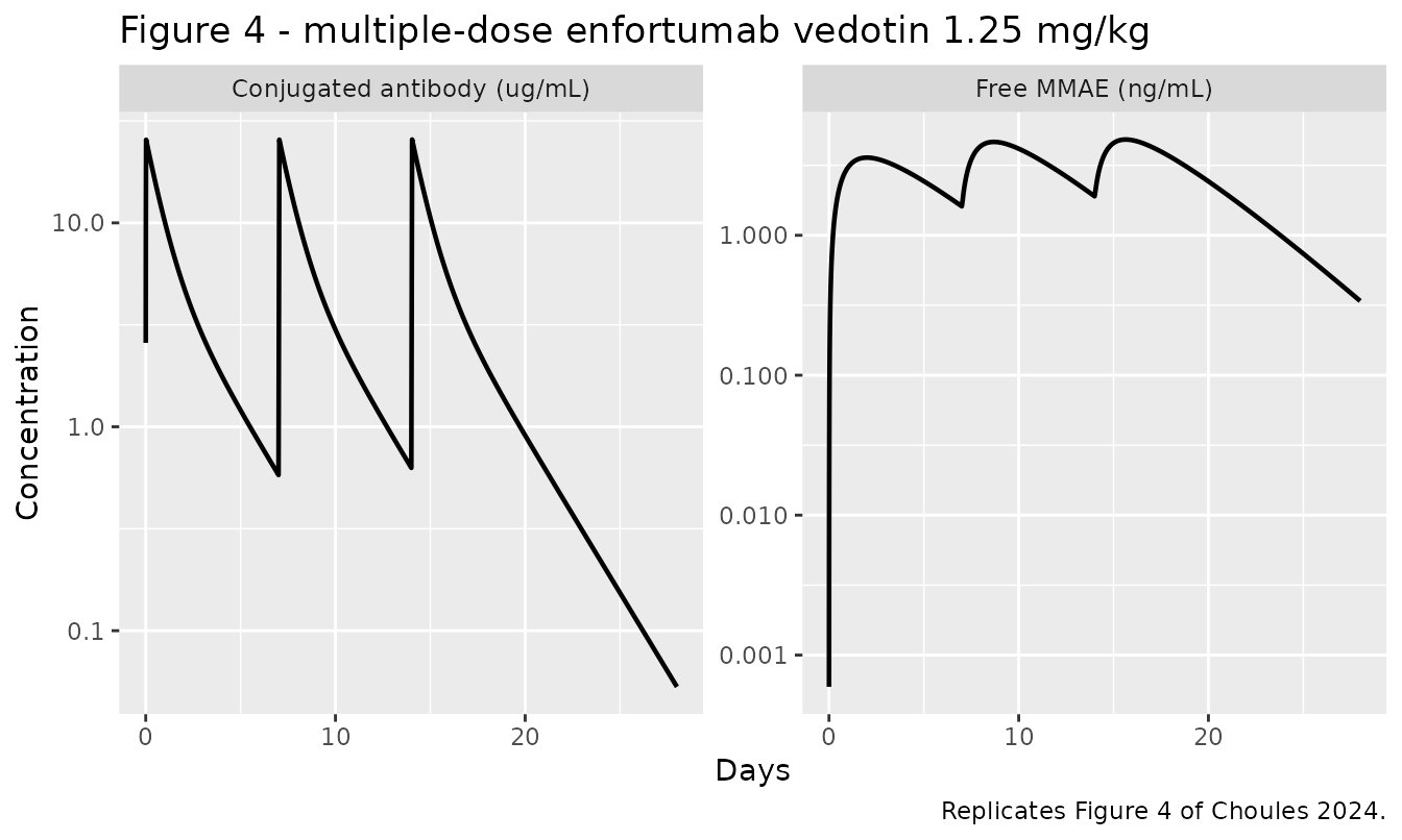

auc_window <- function(d, col, lo, hi) {
  s <- d[d$time >= lo & d$time <= hi, ]
  sum(diff(s$time) * (utils::head(s[[col]], -1) + utils::tail(s[[col]], -1)) / 2)
}
peak_window <- function(d, col, lo, hi) {
  max(d[[col]][d$time >= lo & d$time <= hi], na.rm = TRUE)
}

sim_m <- sim_ev_multi
tab4 <- data.frame(
  Analyte = c("Conjugated antibody", "Conjugated antibody",
              "Conjugated antibody", "Conjugated antibody",
              "Free MMAE", "Free MMAE", "Free MMAE", "Free MMAE"),
  Parameter = c("Day 1 AUC0-7d (ug*day/mL)", "Day 1 Cmax (ug/mL)",
                "Day 15 AUC0-14d (ug*day/mL)", "Day 15 Cmax (ug/mL)",
                "Day 1 AUC0-7d (ng*day/mL)", "Day 1 Cmax (ng/mL)",
                "Day 15 AUC0-14d (ng*day/mL)", "Day 15 Cmax (ng/mL)"),
  Published = c(32.8, 25.4, 37.8, 26.0, 18.1, 3.42, 36.6, 5.00),
  Simulated = c(
    auc_window(sim_m, "Cc", 0, 7 * 24) / 24,
    peak_window(sim_m, "Cc", 0, 24),
    auc_window(sim_m, "Cc", 14 * 24, 28 * 24) / 24,
    peak_window(sim_m, "Cc", 14 * 24, 15 * 24),
    auc_window(sim_m, "Cc_mmae_ng", 0, 7 * 24) / 24,
    peak_window(sim_m, "Cc_mmae_ng", 0, 7 * 24),
    auc_window(sim_m, "Cc_mmae_ng", 14 * 24, 28 * 24) / 24,
    peak_window(sim_m, "Cc_mmae_ng", 14 * 24, 28 * 24)
  )
)
tab4$`% diff` <- round(100 * (tab4$Simulated - tab4$Published) / tab4$Published, 1)
tab4$Simulated <- signif(tab4$Simulated, 3)
knitr::kable(tab4,
             caption = "Multiple-dose holdout: simulated vs Choules 2024 Table 4 (simulated mean). None of these values was used to calibrate the model.")

Multiple-dose holdout: simulated vs Choules 2024 Table 4 (simulated mean). None of these values was used to calibrate the model.

Analyte	Parameter	Published	Simulated	% diff
Conjugated antibody	Day 1 AUC0-7d (ug*day/mL)	32.80	32.60	-0.8
Conjugated antibody	Day 1 Cmax (ug/mL)	25.40	25.60	0.6
Conjugated antibody	Day 15 AUC0-14d (ug*day/mL)	37.80	35.50	-6.0
Conjugated antibody	Day 15 Cmax (ug/mL)	26.00	25.60	-1.4
Free MMAE	Day 1 AUC0-7d (ng*day/mL)	18.10	18.60	2.8
Free MMAE	Day 1 Cmax (ng/mL)	3.42	3.59	5.0
Free MMAE	Day 15 AUC0-14d (ng*day/mL)	36.60	31.60	-13.6
Free MMAE	Day 15 Cmax (ng/mL)	5.00	4.84	-3.3

Brentuximab vedotin (replicates Figure S1 and Table S3)

bv_single <- dplyr::bind_rows(
  make_arm(1L, 1.8, 0, 504, "1.8 mg/kg"),
  make_arm(2L, 2.7, 0, 504, "2.7 mg/kg")
)
sim_bv <- solve_arms(mod_bv, bv_single)
#> Warning: multi-subject simulation without without 'omega'

# Replicates Figure S1 of Choules 2024.
sim_bv |>
  dplyr::filter(time > 0) |>
  dplyr::select(time, treatment, Cc, Cc_mmae_ng) |>
  tidyr::pivot_longer(c(Cc, Cc_mmae_ng), names_to = "analyte",
                      values_to = "conc") |>
  dplyr::mutate(analyte = dplyr::recode(
    analyte,
    Cc = "Conjugated antibody (ug/mL)",
    Cc_mmae_ng = "Free MMAE (ng/mL)"
  )) |>
  ggplot(aes(time / 24, conc, colour = treatment)) +
  geom_line(linewidth = 0.8) +
  facet_wrap(~analyte, scales = "free_y") +
  scale_y_log10() +
  labs(x = "Days", y = "Concentration", colour = NULL,
       title = "Figure S1 - brentuximab vedotin and free MMAE",
       caption = "Replicates Figure S1 of Choules 2024.")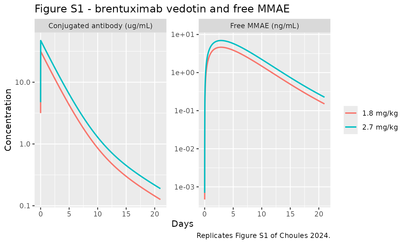

nca_bv_adc <- run_nca(sim_bv, bv_single, "Cc", iv_interval(504, "aucinf.obs"))
ref_bv_adc <- data.frame(
  treatment  = c("1.8 mg/kg", "2.7 mg/kg"),
  cmax       = c(31.5, 47.2),
  aucinf.obs = c(82.2, 123) * 24,
  half.life  = c(5.71, 5.71) * 24
)
tbl_bv_adc <- nlmixr2lib::ncaComparisonTable(
  nca_bv_adc, ref_bv_adc, by = "treatment",
  params = c("cmax", "aucinf.obs", "half.life"),
  units = c(cmax = "ug/mL", aucinf.obs = "ug*h/mL", half.life = "h")
)
knitr::kable(tbl_bv_adc,
             caption = "Conjugated brentuximab vedotin: simulated vs Choules 2024 Table S3 (simulated mean).")

Conjugated brentuximab vedotin: simulated vs Choules 2024 Table S3 (simulated mean).

NCA parameter	treatment	Reference	Simulated	% diff
Cmax (ug/mL)	1.8 mg/kg	31.5	31.5	-0.0%
Cmax (ug/mL)	2.7 mg/kg	47.2	47.2	+0.1%
AUC0-∞ (obs) (ug*h/mL)	1.8 mg/kg	1970	1970	-0.2%
AUC0-∞ (obs) (ug*h/mL)	2.7 mg/kg	2950	2950	+0.0%
t½ (h)	1.8 mg/kg	137	124	-9.3%
t½ (h)	2.7 mg/kg	137	124	-9.3%

attr(tbl_bv_adc, "footnote")
#> NULL

nca_bv_mmae <- run_nca(sim_bv, bv_single, "Cc_mmae_ng",
                       iv_interval(504, "aucinf.obs"))
ref_bv_mmae <- data.frame(
  treatment  = c("1.8 mg/kg", "2.7 mg/kg"),
  cmax       = c(4.62, 6.96),
  aucinf.obs = c(38.5, 58.6) * 24,
  half.life  = c(3.57, 3.56) * 24
)
tbl_bv_mmae <- nlmixr2lib::ncaComparisonTable(
  nca_bv_mmae, ref_bv_mmae, by = "treatment",
  params = c("cmax", "aucinf.obs", "half.life"),
  units = c(cmax = "ng/mL", aucinf.obs = "ng*h/mL", half.life = "h")
)
knitr::kable(tbl_bv_mmae,
             caption = "Free MMAE after brentuximab vedotin: simulated vs Choules 2024 Table S3 (simulated mean). AUC and half-life were held out of the calibration.")

Free MMAE after brentuximab vedotin: simulated vs Choules 2024 Table S3 (simulated mean). AUC and half-life were held out of the calibration.

NCA parameter	treatment	Reference	Simulated	% diff
Cmax (ng/mL)	1.8 mg/kg	4.62	4.63	+0.2%
Cmax (ng/mL)	2.7 mg/kg	6.96	6.94	-0.2%
AUC0-∞ (obs) (ng*h/mL)	1.8 mg/kg	924	926	+0.2%
AUC0-∞ (obs) (ng*h/mL)	2.7 mg/kg	1410	1390	-1.3%
t½ (h)	1.8 mg/kg	85.7	88.6	+3.4%
t½ (h)	2.7 mg/kg	85.4	88.6	+3.7%

attr(tbl_bv_mmae, "footnote")
#> NULL

Drug-drug interaction (replicates Table 5)

The perpetrator effects are encoded as multiplicative factors on MMAE clearance whose magnitudes were set from the published MMAE AUC geometric mean ratios only. The published Cmax ratios were held back, so reproducing them is a zero-free-parameter test of the reduction’s shape.

ddi_arms <- function(mod, dose_mgkg, tmax_h) {
  ev <- dplyr::bind_rows(
    make_arm(1L, dose_mgkg, 0, tmax_h, "ADC alone"),
    make_arm(2L, dose_mgkg, 0, tmax_h, "+ ketoconazole", keto = 1),
    make_arm(3L, dose_mgkg, 0, tmax_h, "+ rifampin", rif = 1)
  )
  s <- solve_arms(mod, ev)
  ref <- s[s$treatment == "ADC alone", ]
  vapply(c("+ ketoconazole", "+ rifampin"), function(tr) {
    a <- s[s$treatment == tr, ]
    c(auc  = auc_window(a, "Cc_mmae_ng", 0, tmax_h) /
             auc_window(ref, "Cc_mmae_ng", 0, tmax_h),
      cmax = max(a$Cc_mmae_ng) / max(ref$Cc_mmae_ng))
  }, numeric(2))
}

# Simulated long enough (as Choules 2024 states) that the AUClast ratio equals
# the AUCinf ratio.
r_ev <- ddi_arms(mod_ev, 1.25, 2000)
#> Warning: multi-subject simulation without without 'omega'
r_bv <- ddi_arms(mod_bv, 1.80, 2000)
#> Warning: multi-subject simulation without without 'omega'

ddi <- data.frame(
  ADC = c(rep("Enfortumab vedotin 1.25 mg/kg", 4),
          rep("Brentuximab vedotin 1.8 mg/kg", 4)),
  Perpetrator = rep(c("Ketoconazole", "Ketoconazole",
                      "Rifampin", "Rifampin"), 2),
  Metric = rep(c("MMAE AUC ratio", "MMAE Cmax ratio"), 4),
  Published = c(1.38, 1.15, 0.47, 0.72,
                1.37, 1.15, 0.47, 0.70),
  Calibrated = rep(c("yes (sets the CL multiplier)", "no (holdout)"), 4),
  Simulated = c(r_ev["auc", 1], r_ev["cmax", 1],
                r_ev["auc", 2], r_ev["cmax", 2],
                r_bv["auc", 1], r_bv["cmax", 1],
                r_bv["auc", 2], r_bv["cmax", 2])
)
ddi$`% diff` <- round(100 * (ddi$Simulated - ddi$Published) / ddi$Published, 1)
ddi$Simulated <- round(ddi$Simulated, 3)
knitr::kable(ddi[, c("ADC", "Perpetrator", "Metric", "Published",
                     "Simulated", "% diff", "Calibrated")],
             caption = "Drug-drug interaction: simulated vs Choules 2024 Table 5 (predicted geometric mean ratios).")

Drug-drug interaction: simulated vs Choules 2024 Table 5 (predicted geometric mean ratios).

ADC	Perpetrator	Metric	Published	Simulated	% diff	Calibrated
Enfortumab vedotin 1.25 mg/kg	Ketoconazole	MMAE AUC ratio	1.38	1.380	0.0	yes (sets the CL multiplier)
Enfortumab vedotin 1.25 mg/kg	Ketoconazole	MMAE Cmax ratio	1.15	1.113	-3.2	no (holdout)
Enfortumab vedotin 1.25 mg/kg	Rifampin	MMAE AUC ratio	0.47	0.470	0.0	yes (sets the CL multiplier)
Enfortumab vedotin 1.25 mg/kg	Rifampin	MMAE Cmax ratio	0.72	0.738	2.6	no (holdout)
Brentuximab vedotin 1.8 mg/kg	Ketoconazole	MMAE AUC ratio	1.37	1.370	0.0	yes (sets the CL multiplier)
Brentuximab vedotin 1.8 mg/kg	Ketoconazole	MMAE Cmax ratio	1.15	1.143	-0.6	no (holdout)
Brentuximab vedotin 1.8 mg/kg	Rifampin	MMAE AUC ratio	0.47	0.470	0.0	yes (sets the CL multiplier)
Brentuximab vedotin 1.8 mg/kg	Rifampin	MMAE Cmax ratio	0.70	0.680	-2.9	no (holdout)

The AUC rows agree by construction. The Cmax rows do not: nothing about them was fitted, and they fall out of the interaction between the ADC-driven MMAE formation rate and the perturbed MMAE elimination rate.

Assumptions and deviations

• The published model is a Simcyp platform PBPK model and these files are a compartmental reduction of it. They reproduce the paper’s predicted plasma concentration-time profiles and exposure metrics for both analytes, and the interaction ratios. They do not reproduce the mechanistic layer: there are no organs, no FcRn recycling, no explicit DAR-isoform species, no gut or hepatic CYP3A4 / P-glycoprotein kinetics, and no tissue MMAE. Use them for exposure simulation, not for mechanistic inference.
• Conjugated-antibody parameters are derived, not transcribed. The four CL / V1 / Q / V2 values per ADC are not printed anywhere in the source; they were solved for from the published simulated summary statistics as described above. Every other value in both files is transcribed directly from the paper.
• Validation targets are the paper’s predictions, not its observed data. The object here is to reproduce the published model, so the calibration and comparison targets throughout are the simulated columns of Tables 3, 4, 5, 6 and S3, never the observed columns.
• Arithmetic means, not geometric means. The simulated curves in Figures 3, 4 and S1 are arithmetic means, so the arithmetic-mean rows are used throughout. The geometric means are 1-2% lower for the conjugated antibody and 7-20% lower for MMAE, because the simulated MMAE distribution is far more skewed (CV up to 79%). A deterministic reduction produces a single profile and cannot reproduce both summaries at once.
• Reference weight 72.0 kg with no body-weight relationship. All parameters are calibrated at the enfortumab vedotin simulated mean weight (Table S4). The paper publishes no weight covariate relationship, and none is identifiable from summary statistics reported at a single population mean weight, so no weight scaling is encoded. Simulating a substantially different body weight will not reproduce Simcyp’s behaviour. Note that MMAE V_ss is printed in L/kg (3.03 L/kg), so a user who wants a different reference individual should rescale lvc_mmae accordingly, but the conjugated-antibody parameters have no such published scaling.
• The brentuximab vedotin population weight is assumed. The source prints no weight for that virtual trial. 72.0 kg is used because both simulations draw from the Simcyp cancer population; the assumption is corroborated by the reduction reproducing the published brentuximab vedotin MMAE AUCinf at both dose levels to within about 1%, which would not happen if the true weight were materially different.
• The released MMAE fraction is 1. F_rel (deconjugation) and F_rel (catabolic) are both 1 in Table 1 and Table S1, so the reduction releases the full stoichiometric payload on antibody elimination. That this reproduces the published MMAE AUC for four dose levels across two ADCs is evidence the assumption is consistent with the source model rather than merely convenient.
• The interaction is a lumped clearance multiplier. Ketoconazole and rifampin act on CYP3A4 and P-glycoprotein in the source, and the rifampin simulation additionally applied a manual fold increase in the P-gp relative activity factor because the simulator did not support transporter induction at the time. All of that is collapsed into a single multiplicative factor on MMAE clearance here. Do not read e_rif_cl_mmae as a CYP3A4 induction magnitude.
• The perpetrator indicators are step functions. The source ran fixed sequence virtual trials in which the perpetrator was dosed daily from before the ADC dose through the end of sampling (Table S2), so no onset or offset kinetics are encoded.
• No residual error and no between-subject variability. Choules 2024 reports neither. The CV% values in Tables 3, 4, 6 and S3 are the spread of the simulated virtual population arising from Simcyp physiological variability, not a residual-error estimate or a population-PK omega, so they are not reused. propSd and propSd_mmae are fixed at 0.
• Half-life is window-sensitive. The published half-lives are non-compartmental estimates over the paper’s own sampling windows (7 days for enfortumab vedotin, 21 days for brentuximab vedotin), not the true terminal half-lives of the underlying model. The NCA above uses the same windows for that reason. The conjugated-antibody parameters were calibrated so that the model’s analytic terminal half-life equals the published value; PKNCA’s automatic terminal-phase selection then lands a few percent away for enfortumab vedotin and about 9% low for brentuximab vedotin, because a 2-compartment reduction and the Simcyp FcRn-recycling model do not curve into their terminal phases at the same rate.
• Accumulation is slightly under-predicted for MMAE. In the multiple-dose holdout, the day-15 MMAE AUC over 14 days is about 14% below the published value while every other row in that table is within 6%. The reduction carries a single MMAE compartment, so it has no slow peripheral pool to accumulate into over three weekly doses. Treat multiple-dose MMAE exposure as a lower bound.

Errata and gaps not covered

• Table 6 labels its predicted conjugated-antibody AUC column as AUCinf, but for enfortumab vedotin it reprints the Table 3 AUC(d0-7) values unchanged (32.2 and 25.7 ug*day/mL, geometric mean). With a 1.94-day half-life the 0-7 day window does not capture the full profile, so the two cannot both be right. This vignette treats those enfortumab vedotin values as AUC(d0-7), matching their Table 3 label. The brentuximab vedotin Table S3 AUC values are labelled AUCinf and are treated as such.
• Midazolam and digoxin are out of scope. The paper also simulated enfortumab vedotin as a perpetrator against midazolam (CYP3A4 substrate) and digoxin (P-glycoprotein substrate), predicting geometric mean ratios of 1.00-1.14, i.e. no clinically relevant effect. Those simulations use the unmodified Simcyp midazolam and digoxin compound files, for which the paper prints no parameters at all, so no victim-drug model can be reconstructed. The finding is a null result and nothing is lost by omitting it.
• The sensitivity analysis is not encoded. Table S5 reports MMAE interaction ratios at biliary clearance fractions of 60%, 70% and 80%; the model files use the 70% base case, which is the value in Table 2. A user can reproduce the other rows by substituting the corresponding e_keto_cl_mmae and e_rif_cl_mmae reciprocals from Table S5.
• Target-mediated drug disposition is absent from the source itself. The authors state that TMDD could not be included due to lack of data, so its absence here is faithful to the published model rather than a simplification introduced by the reduction.