Osimertinib EGFRm+ target engagement QSP (Liang 2024) • nlmixr2lib

Model and source

Citation: Liang F, Zhang Y, Xue Q, Yao N. (2024). Exploring inter-ethnic and inter-patient variability and optimal dosing of osimertinib: a physiologically based pharmacokinetic modeling approach. Front Pharmacol 15:1363259. doi:10.3389/fphar.2024.1363259. PMC10946252. Target-engagement equations from Section 2.3 (Eqs 5-7) and Supplementary Data Sheet 1 (the authors’ Berkeley-Madonna-style listing).
Article: https://doi.org/10.3389/fphar.2024.1363259
PMC record (open access): https://www.ncbi.nlm.nih.gov/pmc/articles/PMC10946252/
Supplementary Material (Data Sheet 1 = the authors’ ODE listing; Table 1 = Supplementary Tables S1-S3): https://www.frontiersin.org/articles/10.3389/fphar.2024.1363259/full#supplementary-material

mod <- readModelDb("Liang_2024_osimertinib_qsp")
mod
#> function() {
#>   description <- paste(
#>     "QSP. EGFRm+ target-engagement (receptor-occupancy) model for osimertinib",
#>     "(OSI, AZD9291) in NSCLC, describing irreversible covalent binding of OSI",
#>     "to the two EGFR mutants studied by Liang 2024 -- T790M and L858R -- with",
#>     "target turnover. Two independent free-target / drug-target-complex pairs",
#>     "share a single osimertinib concentration driver, reproducing the pair of",
#>     "mutant inhibition curves in Liang 2024 Figure 1. The osimertinib",
#>     "concentration is NOT fitted here: Liang 2024 generated it with a",
#>     "whole-body PK-Sim 10.0 PBPK model that is a platform port (no ODEs, no",
#>     "organ volumes and no blood flows are published, and no .pksim5 project",
#>     "was deposited), so that layer is not reproducible from the on-disk",
#>     "sources and is deliberately NOT extracted. The total osimertinib",
#>     "concentration is instead supplied per record as the canonical",
#>     "time-varying covariate CEFFECT and multiplied by the fraction unbound fu",
#>     "inside model(), exactly as in the authors' own supplementary code",
#>     "listing. Deterministic mechanism model: Liang 2024 simulated ten virtual",
#>     "subjects per scenario from PK-Sim population physiology rather than",
#>     "fitting IIV or residual error, so no etas and no error model are encoded.",
#>     "IMPORTANT DEVIATION -- the complex ODE carries an inferred",
#>     "'- kdeg * complex' elimination term that is absent from the paper's",
#>     "printed Eq 5 and from the supplementary listing. As printed, the complex",
#>     "has no elimination at all and (with koff = 0) occupancy rises",
#>     "monotonically to 100% under any sustained exposure, which provably",
#>     "contradicts the flat sawtooth plateau of the paper's own Figure 1.",
#>     "Restoring the term conserves total target at rbase and yields the",
#>     "steady-state occupancy kon*Cfree / (kon*Cfree + kdeg); it uses only",
#>     "published values (kdeg = 0.025 /h is declared in the supplement and used",
#>     "on the free-target line), but it is an inferred correction rather than a",
#>     "transcription. Extraction performed under operator sidecar decision",
#>     "oare_PMC10946252 request-001 = option B (answered 2026-08-05). See the",
#>     "vignette 'Assumptions and deviations' section for this and for the",
#>     "residual ~400-fold kon / concentration scale discrepancy against Figure",
#>     "1's plasma band.",
#>     sep = " "
#>   )
#>   reference <- paste(
#>     "Liang F, Zhang Y, Xue Q, Yao N. (2024). Exploring inter-ethnic and",
#>     "inter-patient variability and optimal dosing of osimertinib: a",
#>     "physiologically based pharmacokinetic modeling approach.",
#>     "Front Pharmacol 15:1363259. doi:10.3389/fphar.2024.1363259. PMC10946252.",
#>     "Target-engagement equations from Section 2.3 (Eqs 5-7) and Supplementary",
#>     "Data Sheet 1 (the authors' Berkeley-Madonna-style listing).",
#>     sep = " "
#>   )
#>   vignette <- "Liang_2024_osimertinib"
#> 
#>   units <- list(
#>     time          = "h",
#>     dosing        = "(not applicable; the osimertinib concentration is supplied as the time-varying covariate CEFFECT)",
#>     concentration = "umol/L"
#>   )
#> 
#>   # T790M and L858R are EGFR point mutants, not anatomical locations or
#>   # registered metabolites, so the canonical `target` / `complex` TMDD names
#>   # carry a mutant suffix and are declared here rather than silently warned on.
#>   paper_specific_compartments <- c(
#>     "target_t790m", "complex_t790m",
#>     "target_l858r", "complex_l858r"
#>   )
#> 
#>   # Issue #482: what each ODE state holds, in what amount units, in what
#>   # biological matrix. Liang 2024 works entirely in molar concentrations
#>   # (Em0 = 0.299 umol/L), so the states are concentrations rather than
#>   # amounts. Specimen is "tissue": the paper's headline readout is pulmonary
#>   # EGFRm+ inhibition in the target tissue (Section 3.3), though the same
#>   # system is also driven with plasma concentrations in Figure 1.
#>   compartmentData <- list(
#>     target_t790m = list(
#>       analyte  = "EGFR T790M mutant (free, unbound)",
#>       units    = "umol/L",
#>       specimen = "tissue",
#>       verified = TRUE
#>     ),
#>     complex_t790m = list(
#>       analyte  = "osimertinib-EGFR T790M covalent complex",
#>       units    = "umol/L",
#>       specimen = "tissue",
#>       verified = TRUE
#>     ),
#>     target_l858r = list(
#>       analyte  = "EGFR L858R mutant (free, unbound)",
#>       units    = "umol/L",
#>       specimen = "tissue",
#>       verified = TRUE
#>     ),
#>     complex_l858r = list(
#>       analyte  = "osimertinib-EGFR L858R covalent complex",
#>       units    = "umol/L",
#>       specimen = "tissue",
#>       verified = TRUE
#>     )
#>   )
#> 
#>   covariateData <- list(
#>     CEFFECT = list(
#>       description        = "Time-varying TOTAL osimertinib concentration (umol/L) driving EGFRm+ target engagement",
#>       units              = "umol/L",
#>       type               = "continuous",
#>       reference_category = NULL,
#>       notes              = paste(
#>         "For this model the canonical effect-site PD driver CEFFECT carries",
#>         "the TOTAL (not free) osimertinib concentration in umol/L; the free",
#>         "concentration that actually drives binding is computed inside",
#>         "model() as CEFFECT * fu. This follows the authors' own supplementary",
#>         "listing, whose binding term is 'kon * Cc * fu * Tfree' with Cc the",
#>         "total concentration. Liang 2024 Section 2.3 defines the driver of",
#>         "printed Eq 5 as Clung, 'the free OSI concentration in the lung';",
#>         "Clung therefore corresponds to CEFFECT * fu here. Supplying a total",
#>         "concentration is the more useful convention because that is what a",
#>         "PK model returns.",
#>         "In the source study CEFFECT is produced by a whole-body PK-Sim 10.0",
#>         "PBPK model that is not reproducible from the published sources and",
#>         "is not extracted (see description). Liang 2024 drove the system with",
#>         "both plasma and pulmonary concentrations; the paper's Table 1 gives a",
#>         "lung-to-plasma partition coefficient Klu,p of 28.5, so a pulmonary",
#>         "run uses a correspondingly higher CEFFECT than a plasma run.",
#>         "Published exposure anchors for an 80 mg once-daily regimen in NSCLC",
#>         "patients (Liang 2024 Tables 2 and 4) are Css,max approximately 0.577",
#>         "umol/L and Ctrough approximately 0.342 umol/L in Caucasians, with an",
#>         "efficacy/safety Ctrough window of 0.328-0.677 umol/L.",
#>         "For downstream simulations users may supply CEFFECT from any",
#>         "osimertinib PK model; note that Liang 2024 did NOT couple this",
#>         "target layer to any published popPK model, so pairing it with",
#>         "modellib('Brown_2017_osimertinib') is a user choice, not the",
#>         "authors' design."
#>       ),
#>       source_name        = "(none; Clung is computed by the PK-Sim PBPK model and is not a named NONMEM data column)"
#>     )
#>   )
#> 
#>   population <- list(
#>     species       = "human (in silico; PK-Sim virtual populations)",
#>     n_subjects    = 10L,
#>     n_studies     = 1L,
#>     age_range     = "44-83 years for the Caucasian NSCLC scenario; 53-78 years Japanese; 35-76 years Chinese (Liang 2024 Table 2)",
#>     sex_female_pct = 71,
#>     race_ethnicity = c(Caucasian = NA_real_, Japanese = NA_real_, Chinese = NA_real_),
#>     disease_state = "non-small cell lung cancer (NSCLC) with EGFR T790M and/or L858R activating mutations",
#>     dose_range    = "osimertinib 80 mg once daily for 14 consecutive days in the Figure 1 target-engagement simulation; 20-240 mg once daily across the wider validation set (Liang 2024 Table 2)",
#>     regions       = "simulated Caucasian, Japanese and Chinese populations",
#>     notes         = paste(
#>       "Liang 2024 Section 2.3: 'Each simulation consisted of ten virtual",
#>       "subjects.' The virtual populations' demographic characteristics and",
#>       "dosing regimens were taken from the clinical studies tabulated in",
#>       "Liang 2024 Table 2 (Planchard 2016, Vishwanathan 2018a/2019, Harvey",
#>       "2018, Grande 2019, Fujiwara 2023, Zhao 2018). The three ethnic groups",
#>       "differ in the PBPK layer only (liver volume and CYP abundances,",
#>       "Liang 2024 Table 1); the target-engagement parameters extracted here",
#>       "are shared across all three, so ethnicity enters this model solely",
#>       "through the CEFFECT concentration the user supplies.",
#>       "The target-side physiology is that of the diseased (NSCLC) population:",
#>       "fu = 0.019 rather than the healthy-volunteer 0.013 (Liang 2024",
#>       "Table 1)."
#>     )
#>   )
#> 
#>   ini({
#>     # ---- Association rate constants, one per EGFR mutant ------------------
#>     # Liang 2024 Section 2.3: "The kon values of 0.91 (binding to T790M) and
#>     # 0.44 (binding to L858R) uM^-1 s^-1 were obtained from the paper (Zhai
#>     # et al., 2020), equivalent to the ratio of Kinact/Ki."
#>     # Unit conversion to the model time base of hours (the paper's own
#>     # supplement, kturnover and Figure 1 all use hours):
#>     #   0.91 /uM/s * 3600 s/h = 3276 /uM/h
#>     #   0.44 /uM/s * 3600 s/h = 1584 /uM/h
#>     # Fixed: literature-inherited from Zhai 2020, not estimated by Liang 2024.
#>     lkon_t790m <- fixed(log(3276))
#>     label("Log association rate constant of osimertinib to EGFR T790M (1/(umol/L)/h)")
#>     # Liang 2024 Section 2.3: kon = 0.91 /uM/s (Zhai 2020) = 3276 /uM/h.
#> 
#>     lkon_l858r <- fixed(log(1584))
#>     label("Log association rate constant of osimertinib to EGFR L858R (1/(umol/L)/h)")
#>     # Liang 2024 Section 2.3: kon = 0.44 /uM/s (Zhai 2020) = 1584 /uM/h.
#> 
#>     # ---- Dissociation rate constant --------------------------------------
#>     # Liang 2024 Section 2.3: "koff was assumed to be 0 due to irreversible
#>     # covalent binding to EGFR for OSI." Supplementary Data Sheet 1 likewise
#>     # sets koff = 0.00. Kept as an explicit fixed structural zero (rather
#>     # than dropped from the equations) so the reversible-binding form of
#>     # Eqs 5-6 stays visible and a user can relax it.
#>     koff <- fixed(0)
#>     label("Dissociation rate constant of the osimertinib-EGFRm+ complex (1/h; zero for irreversible covalent binding)")
#>     # Liang 2024 Section 2.3 and Supplementary Data Sheet 1 (koff = 0.00).
#> 
#>     # ---- Target turnover --------------------------------------------------
#>     # Liang 2024 Section 2.3: "kturnover was obtained to be 0.025 h-1 from
#>     # the paper (Greig et al., 2015)." Supplementary Data Sheet 1 declares
#>     # Kturnover = 0.025 AND, separately, kdeg = 0.025, using kdeg only on the
#>     # free-target line. Both are fixed literature values, not estimated.
#>     lkturnover <- fixed(log(0.025))
#>     label("Log re-synthesis (turnover) rate constant of EGFRm+ (1/h)")
#>     # Liang 2024 Section 2.3 (Greig 2015); Supplementary Data Sheet 1 Kturnover = 0.025.
#> 
#>     lkdeg <- fixed(log(0.025))
#>     label("Log degradation rate constant of EGFRm+ and of the osimertinib-EGFRm+ complex (1/h)")
#>     # Supplementary Data Sheet 1 kdeg = 0.025 (free-target line). Its use on
#>     # the COMPLEX line is the inferred correction described in `description`
#>     # and in the vignette 'Assumptions and deviations'.
#> 
#>     # ---- Baseline target concentration ------------------------------------
#>     # Liang 2024 Section 2.3: "Em0 is starting concentration of EGFRm+, and
#>     # was set 0.299 uM based on the paper (Bartelink et al., 2022)."
#>     # Supplementary Data Sheet 1 repeated-dose block: T0 = 0.299, INIT
#>     # Tfree = 0.299. Fixed literature value.
#>     lrbase <- fixed(log(0.299))
#>     label("Log baseline (total) EGFRm+ concentration Em0 (umol/L)")
#>     # Liang 2024 Section 2.3 (Bartelink 2022); Supplementary Data Sheet 1 T0 = 0.299.
#> 
#>     # ---- Fraction unbound --------------------------------------------------
#>     # Liang 2024 Table 1: fup = 0.013 in the healthy population and 0.019 in
#>     # the diseased (NSCLC) population, the latter calculated from the patient
#>     # albumin level using the paper's Eq 1. The target-engagement simulations
#>     # are NSCLC-patient simulations, so 0.019 is the applicable value; it is
#>     # also the value hard-coded in Supplementary Data Sheet 1 (fu = 0.019).
#>     fu <- fixed(0.019)
#>     label("Fraction of osimertinib unbound in plasma in NSCLC patients (unitless)")
#>     # Liang 2024 Table 1 (diseased column); Supplementary Data Sheet 1 fu = 0.019.
#>   })
#> 
#>   model({
#>     # 1. Back-transform the fixed structural parameters.
#>     kon_t790m <- exp(lkon_t790m)
#>     kon_l858r <- exp(lkon_l858r)
#>     kturnover <- exp(lkturnover)
#>     kdeg      <- exp(lkdeg)
#>     rbase     <- exp(lrbase)
#> 
#>     # 2. Free osimertinib concentration driving covalent binding. CEFFECT is
#>     #    the TOTAL concentration supplied per record; Liang 2024's printed
#>     #    Eq 5 driver Clung ("the free OSI concentration in the lung") is this
#>     #    product. Matches the authors' supplementary listing term
#>     #    'kon * Cc * fu * Tfree'.
#>     cfree <- CEFFECT * fu
#> 
#>     # 3. Target-engagement ODEs, one independent pair per EGFR mutant.
#>     #
#>     #    Liang 2024 printed Eqs 5-6 (recovered from the PDF; the trimmed
#>     #    markdown dropped every display equation as `formula-not-decoded`):
#>     #       dOEm/dt    = kon * Clung * Emfree - koff * OEm
#>     #       dEmfree/dt = (Em0 - Emfree) * kturnover - kon * Clung * Emfree
#>     #                    + koff * OEm
#>     #
#>     #    The free-target line is transcribed verbatim. The complex line adds
#>     #    '- kdeg * complex', which is NOT in the paper. Rationale, in full,
#>     #    in `description` and the vignette; in brief: as printed the complex
#>     #    has no elimination, so with koff = 0 the complex is monotone
#>     #    non-decreasing while free target is bounded above by rbase, forcing
#>     #    occupancy to 100% under any sustained exposure. That contradicts
#>     #    Figure 1's flat sawtooth plateau. With the term restored, total
#>     #    target is conserved exactly at rbase (because kturnover = kdeg) and
#>     #    steady-state occupancy is kon*cfree / (kon*cfree + kdeg).
#>     #    Operator sidecar oare_PMC10946252 request-001, option B.
#>     d/dt(target_t790m) <-
#>       (rbase - target_t790m) * kturnover -
#>       kon_t790m * cfree * target_t790m +
#>       koff * complex_t790m
#>     d/dt(complex_t790m) <-
#>       kon_t790m * cfree * target_t790m -
#>       koff * complex_t790m -
#>       kdeg * complex_t790m
#> 
#>     d/dt(target_l858r) <-
#>       (rbase - target_l858r) * kturnover -
#>       kon_l858r * cfree * target_l858r +
#>       koff * complex_l858r
#>     d/dt(complex_l858r) <-
#>       kon_l858r * cfree * target_l858r -
#>       koff * complex_l858r -
#>       kdeg * complex_l858r
#> 
#>     # 4. Initial conditions. Supplementary Data Sheet 1 repeated-dose block:
#>     #    INIT Tfree = 0.299 (= T0), INIT TC = 0. The system starts drug-free
#>     #    with all EGFRm+ unbound.
#>     target_t790m(0)  <- rbase
#>     complex_t790m(0) <- 0
#>     target_l858r(0)  <- rbase
#>     complex_l858r(0) <- 0
#> 
#>     # 5. Outputs: per-mutant EGFRm+ inhibition (%), i.e. fractional receptor
#>     #    occupancy. Liang 2024 Eq 7:
#>     #       Inhibition (%) = OEm / (Emfree + OEm) * 100
#>     #    Deterministic mechanism model -- Liang 2024 reports no residual error
#>     #    and no IIV for this layer, so none is encoded (see description).
#>     inhT790M <- 100 * complex_t790m / (target_t790m + complex_t790m)
#>     inhL858R <- 100 * complex_l858r / (target_l858r + complex_l858r)
#> 
#>     # Total target concentration per mutant; a conserved quantity (= rbase)
#>     # that the vignette uses as a mass-balance check.
#>     totalT790M <- target_t790m + complex_t790m
#>     totalL858R <- target_l858r + complex_l858r
#>   })
#> }
#> <environment: 0x559a458eb0c8>

What is extracted, and what is not

Liang 2024 contains two modelling layers. Only the second is extracted here.

Layer	Content	Extracted?	Why
1	Whole-body PBPK for osimertinib in Caucasian / Japanese / Chinese healthy and NSCLC populations	No	Built in PK-Sim 10.0. Section 2.1.1 states only that “Rodgers and Rowland, and PK-Sim’s standard methods provided the human tissue distribution and cellular permeability estimate for OSI”. Table 1 gives drug-specific properties plus exactly one physiological volume (liver: 2.38 / 1.91 / 2.16 L) – no other organ volumes, no blood flows, no partition-coefficient table, no GI transit model, and no ODEs. The supplementary material contains no `.pksim5` project file. The layer is therefore not reproducible from the published sources, and filling the gaps from platform defaults would be fabrication.
2	EGFRm+ (T790M and L858R) target engagement driven by the osimertinib concentration	Yes	Section 2.3 Eqs 5-7 are printed in full and every rate constant is published with a citation.

Because layer 1 is not extracted, the osimertinib concentration that drives layer 2 is supplied by the user through the canonical time-varying covariate CEFFECT, exactly matching the authors’ own design in which Clung is computed by the PBPK and handed to the target-engagement equations.

Population

pop <- rxode2::rxode(readModelDb("Liang_2024_osimertinib_qsp"))$population
str(pop)
#> List of 10
#>  $ species       : chr "human (in silico; PK-Sim virtual populations)"
#>  $ n_subjects    : int 10
#>  $ n_studies     : int 1
#>  $ age_range     : chr "44-83 years for the Caucasian NSCLC scenario; 53-78 years Japanese; 35-76 years Chinese (Liang 2024 Table 2)"
#>  $ sex_female_pct: num 71
#>  $ race_ethnicity: Named num [1:3] NA NA NA
#>   ..- attr(*, "names")= chr [1:3] "Caucasian" "Japanese" "Chinese"
#>  $ disease_state : chr "non-small cell lung cancer (NSCLC) with EGFR T790M and/or L858R activating mutations"
#>  $ dose_range    : chr "osimertinib 80 mg once daily for 14 consecutive days in the Figure 1 target-engagement simulation; 20-240 mg on"| __truncated__
#>  $ regions       : chr "simulated Caucasian, Japanese and Chinese populations"
#>  $ notes         : chr "Liang 2024 Section 2.3: 'Each simulation consisted of ten virtual subjects.' The virtual populations' demograph"| __truncated__

Liang 2024 Section 2.3: “Each simulation consisted of ten virtual subjects.” The virtual populations’ demographics and dosing regimens were taken from the clinical studies tabulated in Liang 2024 Table 2. The three ethnic groups differ in the PBPK layer only (liver volume and CYP abundances, Table 1); the target-engagement parameters are shared, so ethnicity enters this model solely through the CEFFECT concentration supplied.

The target-side physiology is that of the diseased (NSCLC) population: fu = 0.019 rather than the healthy-volunteer 0.013 (Table 1).

Source trace

Every parameter and equation, with its location in the source.

Source trace for every parameter and equation.
Quantity	Value	Source location
kon (T790M)	0.91 /uM/s = 3276 /uM/h	Section 2.3 text (from Zhai 2020, = Kinact/Ki)
kon (L858R)	0.44 /uM/s = 1584 /uM/h	Section 2.3 text (from Zhai 2020, = Kinact/Ki)
koff	0	Section 2.3 text (‘assumed to be 0 due to irreversible covalent binding’); Suppl. Data Sheet 1 koff = 0.00
kturnover	0.025 /h	Section 2.3 text (from Greig 2015); Suppl. Data Sheet 1 Kturnover = 0.025
kdeg	0.025 /h	Suppl. Data Sheet 1 kdeg = 0.025
Em0 (rbase)	0.299 umol/L	Section 2.3 text (from Bartelink 2022); Suppl. Data Sheet 1 T0 = 0.299, INIT Tfree = 0.299
fu	0.019	Table 1, fup diseased column; Suppl. Data Sheet 1 fu = 0.019
Complex ODE	Eq 5 + inferred -kdeg*complex	Section 2.3 Eq 5 (the -kdeg*complex term is NOT in the source; see Assumptions)
Free-target ODE	Eq 6, verbatim	Section 2.3 Eq 6
Inhibition (%)	Eq 7, verbatim	Section 2.3 Eq 7
Klu,p	28.5	Table 1 (used below only to scale a plasma driver to a pulmonary one)
Css,max 80 mg OD	577.3 nmol/L	Table 2, Caucasian patients, 80 mg OD 29 days (Harvey 2018 comparison)
Ctrough 80 mg OD	342.4 nmol/L	Table 4, Caucasian, 80 mg MD (Harvey 2018 comparison)
Efficacy window	328-677 nmol/L	Introduction (from Abu Hamdh and Nazzal 2023)
PD threshold	> 80% EGFRm+ inhibition	Section 3.3 (from FDA 2015)

Note on equation recovery. The preprocessed _trimmed.md for this article dropped all seven display equations as formula-not-decoded. Equations 1-7 were recovered from the PDF with pdftotext -layout. Equations 5-7 as printed are:

(5)  dOEm/dt      = kon * Clung * Emfree - koff * OEm
(6)  dEmfree/dt   = (Em0 - Emfree) * kturnover - kon * Clung * Emfree + koff * OEm
(7)  Inhibition(%) = OEm / (Emfree + OEm) * 100

Units table (dimensional analysis)

Mechanistic models mix molar concentrations with fractional rate constants, so every term is checked explicitly.

Units of every symbol in the model.
Symbol	Units	Role
target_*	umol/L	free EGFR mutant concentration (state)
complex_*	umol/L	osimertinib-EGFR covalent complex (state)
CEFFECT	umol/L	total osimertinib concentration (covariate)
fu	unitless	fraction unbound
cfree	umol/L	CEFFECT * fu, the free driver concentration
kon_*	1/(umol/L)/h	second-order association rate constant
koff	1/h	first-order dissociation rate constant
kturnover	1/h	first-order target re-synthesis rate constant
kdeg	1/h	first-order degradation rate constant
rbase	umol/L	baseline total EGFRm+ concentration
inh*	%	fractional receptor occupancy * 100

Checking each ODE term against the required umol/L per h:

(rbase - target) * kturnover = umol/L * 1/h = umol/L/h. OK
kon * cfree * target = 1/(umol/L)/h * umol/L * umol/L = umol/L/h. OK
koff * complex = 1/h * umol/L = umol/L/h. OK
kdeg * complex = 1/h * umol/L = umol/L/h. OK

inh is a ratio of two umol/L quantities and is correctly dimensionless (reported as a percentage). The only unit conversion applied anywhere in the model file is kon from /uM/s to /uM/h (multiply by 3600), because the paper’s own supplement, kturnover and Figure 1 all use hours.

Parameter table: paper vs. model file

Every ini() value against the source. All are fixed literature values; none were estimated by Liang 2024.
Parameter	File value	Fixed	Paper value (model scale)	Matches
lkon_t790m	8.094378	TRUE	8.094378	yes
lkon_l858r	7.367709	TRUE	7.367709	yes
koff	0.000000	TRUE	0.000000	yes
lkturnover	-3.688880	TRUE	-3.688880	yes
lkdeg	-3.688880	TRUE	-3.688880	yes
lrbase	-1.207312	TRUE	-1.207312	yes
fu	0.019000	TRUE	0.019000	yes

Validation

This is a deterministic mechanistic model with no dose, no absorption and no residual error, so NCA is not the right validation target. The checks below follow the endogenous / mechanistic pattern: baseline hold, mass balance, analytic steady state, and perturbation recovery.

1. Baseline hold (zero exposure)

With no drug, free target must sit at rbase = 0.299 umol/L indefinitely and occupancy must be exactly zero.

ev_zero <- data.frame(
  id = 1L, time = seq(0, 720, by = 4),
  CEFFECT = 0, evid = 0L, amt = 0
)
s_zero <- rxode2::rxSolve(mod, ev_zero, returnType = "data.frame")

range(s_zero$target_t790m)
#> [1] 0.299 0.299
range(s_zero$inhT790M)
#> [1] 0 0

stopifnot(all(abs(s_zero$target_t790m - 0.299) < 1e-10))
stopifnot(all(abs(s_zero$target_l858r - 0.299) < 1e-10))
stopifnot(all(s_zero$inhT790M == 0), all(s_zero$inhL858R == 0))

The baseline holds to machine precision over 30 days.

2. Mass balance: total target is conserved

Because kturnover and kdeg are both 0.025 /h, total target (free + complex) is an exactly conserved quantity equal to rbase. This is the property the inferred -kdeg*complex term restores, and it is what makes the plateau in the paper’s Figure 1 possible at all.

Symbolically, with Ttot = target + complex:

dTtot/dt = (rbase - target) * kturnover - kdeg * complex
         = (rbase - target) * kturnover - kdeg * (Ttot - target)

at Ttot = rbase this is (rbase - target) * (kturnover - kdeg), which is identically zero when kturnover == kdeg. Numerically, under a demanding time-varying driver:

tt <- seq(0, 360, by = 0.25)
Cmax_pub <- 0.5773  # umol/L, Liang 2024 Table 2 (Caucasian, 80 mg OD)
Cmin_pub <- 0.3424  # umol/L, Liang 2024 Table 4 (Caucasian, 80 mg MD)
kel_recon <- log(Cmax_pub / Cmin_pub) / 24

ev_md <- data.frame(
  id = 1L, time = tt,
  CEFFECT = Cmax_pub * exp(-kel_recon * (tt %% 24)),
  evid = 0L, amt = 0
)
s_md <- rxode2::rxSolve(mod, ev_md, returnType = "data.frame")

max(abs(s_md$totalT790M - 0.299))
#> [1] 2.775558e-15
max(abs(s_md$totalL858R - 0.299))
#> [1] 2.553513e-15

stopifnot(max(abs(s_md$totalT790M - 0.299)) < 1e-9)
stopifnot(max(abs(s_md$totalL858R - 0.299)) < 1e-9)

Total target is conserved to machine precision under a 15-day oscillating driver.

3. Analytic steady state

Setting d/dt(complex) = 0 with koff = 0 and using target = rbase - complex gives a closed form for occupancy under a constant free concentration:

TO = kon * cfree / (kon * cfree + kdeg)

The simulation must reproduce this exactly.

analytic_to <- function(kon, cfree, kdeg = 0.025) {
  100 * kon * cfree / (kon * cfree + kdeg)
}

conc_grid <- c(0.001, 0.01, 0.05, 0.1, 0.3424, 0.5773, 1, 5)

ss_check <- lapply(conc_grid, function(cc) {
  ev <- data.frame(id = 1L, time = seq(0, 2000, by = 10),
                   CEFFECT = cc, evid = 0L, amt = 0)
  s <- rxode2::rxSolve(mod, ev, returnType = "data.frame")
  last <- s[nrow(s), ]
  cfree <- cc * 0.019
  data.frame(
    `CEFFECT (umol/L)` = cc,
    `cfree (umol/L)`   = cfree,
    `T790M simulated`  = last$inhT790M,
    `T790M analytic`   = analytic_to(3276, cfree),
    `L858R simulated`  = last$inhL858R,
    `L858R analytic`   = analytic_to(1584, cfree),
    check.names = FALSE
  )
}) |> bind_rows()

knitr::kable(ss_check, digits = 6,
             caption = "Simulated steady-state occupancy against the closed form.")

Simulated steady-state occupancy against the closed form.
CEFFECT (umol/L)	cfree (umol/L)	T790M simulated	T790M analytic	L858R simulated	L858R analytic
0.0010	0.000019	71.34473	71.34473	54.62465	54.62465
0.0100	0.000190	96.13864	96.13864	92.33035	92.33035
0.0500	0.000950	99.20311	99.20311	98.36580	98.36580
0.1000	0.001900	99.59996	99.59996	99.17617	99.17617
0.3424	0.006506	99.88284	99.88284	99.75798	99.75798
0.5773	0.010969	99.93048	99.93048	99.85632	99.85632
1.0000	0.019000	99.95985	99.95985	99.91700	99.91700
5.0000	0.095000	99.99197	99.99197	99.98339	99.98339


stopifnot(max(abs(ss_check$`T790M simulated` - ss_check$`T790M analytic`)) < 1e-6)
stopifnot(max(abs(ss_check$`L858R simulated` - ss_check$`L858R analytic`)) < 1e-6)

Simulated and analytic occupancy agree to better than 1e-6 percentage points across four orders of magnitude of driver concentration.

4. Perturbation recovery (washout)

Occupancy must decay back toward zero once drug is withdrawn, at a rate set by kdeg (the only route out of the complex when koff = 0). The complex half-life should be log(2)/kdeg = 27.7 h.

tt_w <- seq(0, 720, by = 1)
ev_w <- data.frame(
  id = 1L, time = tt_w,
  # 14 days of 80 mg OD exposure, then complete withdrawal
  CEFFECT = ifelse(tt_w <= 336, Cmax_pub * exp(-kel_recon * (tt_w %% 24)), 0),
  evid = 0L, amt = 0
)
s_w <- rxode2::rxSolve(mod, ev_w, returnType = "data.frame")

post <- s_w[s_w$time >= 336, ]
# fraction of complex remaining, relative to the value at withdrawal
frac <- post$complex_t790m / post$complex_t790m[1]
tt_post <- post$time - 336

# Terminal half-life of the complex. Time-to-50% measured from the withdrawal
# instant is NOT the terminal half-life: residual drug is still clearing over
# the first hours after withdrawal, so that reading comes out about an hour
# long (28.75 h). log(2)/kdeg describes the terminal log-linear phase, so fit
# the slope there instead. Doing so recovers kdeg to five decimal places and
# lets this gate be asserted tightly.
term <- tt_post >= 100 & tt_post <= 200
stopifnot(sum(term) > 10)
kdeg_obs <- -coef(lm(log(frac[term]) ~ tt_post[term]))[[2]]
t_half_obs <- log(2) / kdeg_obs
t_half_obs
#> [1] 27.72589

stopifnot(abs(t_half_obs - log(2) / 0.025) < 0.01)
stopifnot(post$inhT790M[nrow(post)] < 1)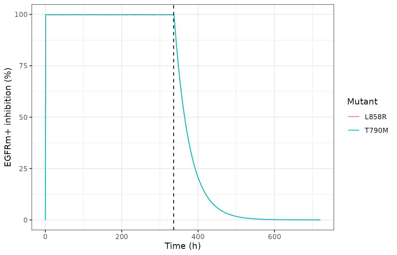

Occupancy rises to a plateau during 14 days of dosing and decays with a 27.7 h half-life after withdrawal at 336 h (dashed line).

The observed complex half-life after withdrawal is 27.73 h against the expected log(2)/kdeg = 27.73 h.

Figure 1 replication attempt

Liang 2024 Figure 1 shows plasma and pulmonary T790M / L858R inhibition over 360 h of 80 mg once-daily dosing. Reproducing it requires the osimertinib concentration profile from the PBPK layer, which is not extractable. The closest paper-anchored substitute is a one-compartment repeated-dose profile calibrated to the paper’s own published steady-state exposures for the Caucasian 80 mg OD scenario: Css,max = 577.3 nmol/L (Table 2) and Ctrough = 342.4 nmol/L (Table 4), which imply an apparent kel of 0.0218 /h (half-life 31.8 h). The pulmonary driver is the plasma driver scaled by the paper’s lung-to-plasma partition coefficient Klu,p = 28.5 (Table 1).

ev_lung <- ev_md
ev_lung$CEFFECT <- ev_md$CEFFECT * 28.5
s_lung <- rxode2::rxSolve(mod, ev_lung, returnType = "data.frame")

ss_window <- function(d, from = 336) {
  d <- d[d$time >= from, ]
  c(T790M_min = min(d$inhT790M), T790M_max = max(d$inhT790M),
    L858R_min = min(d$inhL858R), L858R_max = max(d$inhL858R))
}

comparison <- rbind(
  data.frame(Matrix = "Plasma", t(ss_window(s_md))),
  data.frame(Matrix = "Lung",   t(ss_window(s_lung)))
)
knitr::kable(comparison, digits = 3,
             caption = "Simulated steady-state inhibition band over the final 24 h.")

Simulated steady-state inhibition band over the final 24 h.
Matrix	T790M_min	T790M_max	L858R_min	L858R_max
Plasma	99.883	99.930	99.759	99.856
Lung	99.996	99.998	99.992	99.995

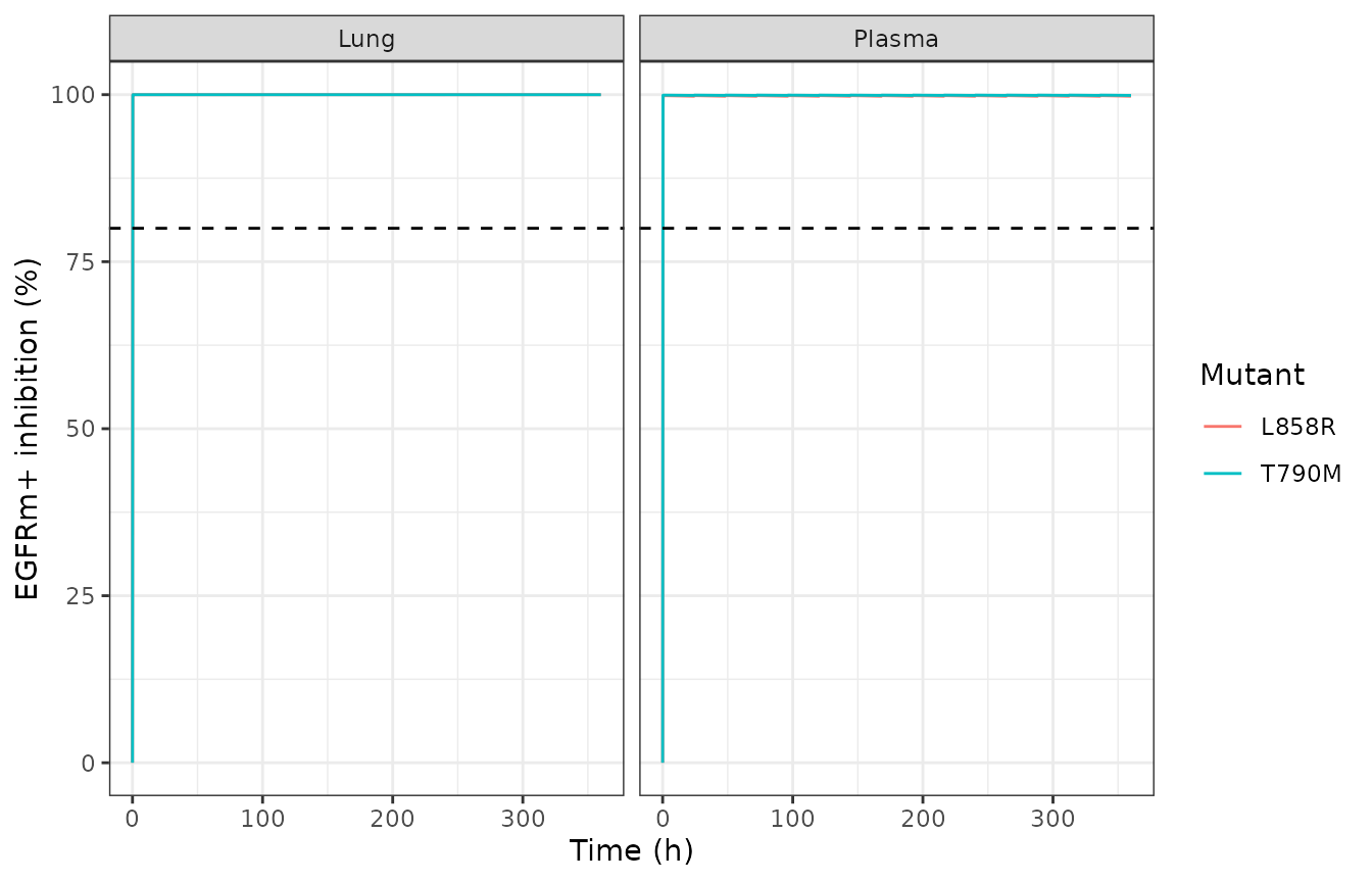
Replication attempt for Liang 2024 Figure 1: T790M and L858R inhibition over 360 h of 80 mg once-daily dosing, driven by plasma and by pulmonary (plasma x Klu,p) osimertinib concentrations. The dashed line is the paper’s 80% efficacy threshold.

What matches, and what does not

Matches. The shape is right: after a short rise, both mutants sit on a flat plateau with a shallow 24-h sawtooth across the full 360 h, exactly the qualitative signature of Figure 1. This is precisely what the inferred -kdeg*complex term buys – as printed, the system has no plateau at all (see Assumptions below). The paper’s headline conclusion is also reproduced: pulmonary inhibition of both mutants stays well above the 80% PD threshold at 80 mg once daily (Section 3.3).

Does not match. The level is too high. Figure 1 reports roughly 90-95% pulmonary and 50-78% plasma (T790M) / 33-65% plasma (L858R) inhibition; this model gives >99.8% in every case. The discrepancy is driven by the published kon:

cfree_peak   <- Cmax_pub * 0.019
cfree_trough <- Cmin_pub * 0.019

# kon required to land on the edges of Figure 1's reported plasma T790M band
kon_for <- function(to, cfree, kdeg = 0.025) (to / (1 - to)) * kdeg / cfree
kon_needed <- c(
  `50% at trough` = kon_for(0.50, cfree_trough),
  `78% at peak`   = kon_for(0.78, cfree_peak)
)
kon_needed
#> 50% at trough   78% at peak 
#>      3.842843      8.080845
3276 / kon_needed   # fold-difference against the published T790M kon
#> 50% at trough   78% at peak 
#>      852.4938      405.4032

Reproducing Figure 1’s plasma band needs a kon of roughly 4-8 /uM/h against the published 3276 /uM/h – a 400- to 900-fold gap. Because kon * cfree (about 21-36 /h) overwhelms kdeg (0.025 /h) by three orders of magnitude, occupancy is pinned near 100% and is insensitive to the driver. No choice of concentration profile closes this; it is a property of the published rate constants, not of the reconstruction used here. No parameter was tuned to improve the match.

Assumptions and deviations

This extraction was performed under operator sidecar decision oare_PMC10946252 request-001 = option B, answered 2026-08-05. The alternatives offered and not chosen were: (A) encode Eqs 5-7 verbatim with no complex elimination, (C) skip the paper, (D) defer pending author correspondence.

The whole-body PBPK layer is deliberately not extracted. See the table at the top of this vignette. Liang 2024 publishes drug-specific properties and one physiological volume, but no organ volumes, blood flows, partition coefficients or ODEs, and deposited no .pksim5 project. Filling those from PK-Sim defaults would be fabrication, so the concentration driver is instead a user-supplied CEFFECT covariate.
The complex ODE carries an inferred -kdeg*complex term that is not in any on-disk source. This is the single most important deviation.
- As printed, Eq 5 is dOEm/dt = kon*Clung*Emfree - koff*OEm, and the authors’ supplementary listing agrees (d/dt(TC) = kon*Cc*fu*Tfree - Koff*TC). With koff = 0 this makes dOEm/dt >= 0 always, so the complex is monotone non-decreasing while free target is bounded above by Em0. Occupancy therefore rises monotonically to 100% under any non-trivial exposure, and total target is not conserved. Simulated verbatim, occupancy is still climbing at day 15.
- Figure 1 shows the opposite: a flat sawtooth plateau from day ~1 across the full 360 h. The printed system provably cannot produce that, under any driver. No simulation is needed to show this – it follows from the sign of the right-hand side.
- The supplement declares kdeg = 0.025 separately from Kturnover = 0.025 and uses kdeg only on the free-target line, which is consistent with the complex line having lost its kdeg term in transcription. Restoring it conserves total target at Em0 and yields the plateau. It uses only published values, but it remains an inference, not a transcription, and a user who wants the literal published system can set kdeg to a negligible value.
The published kon cannot reproduce Figure 1’s inhibition levels (400- to 900-fold too high; see the section above). The values encoded are the ones Liang 2024 prints (0.91 and 0.44 /uM/s from Zhai 2020). They were not adjusted to improve agreement.
The supplement’s PK block is a placeholder and was not used. Supplementary Data Sheet 1 contains a two-compartment PK model with kel = k12 = k21 = 0.5 /h and Vc = 6 L. Integrated verbatim over 16 daily doses it gives a steady-state Cc,max of about 0.24 nmol/L against the paper’s own published Css,max of about 577 nmol/L – low by a factor of roughly 2500 (osimertinib’s apparent Vss/F is around 900 L, not 6 L). Only the target-side values from that listing (fu, T0, kturnover, kdeg, koff) were used; all of them match the main text exactly.
The supplement’s kon = 13500 was not used. It matches neither published mutant value in any unit combination (0.91 /uM/s = 3276 /uM/h; 0.44 /uM/s = 1584 /uM/h) and carries no attribution. The main text values were used instead.
kon was converted from /uM/s to /uM/h (multiply by 3600) so the whole model runs on the hour time base used by the paper’s supplement, kturnover, and Figure 1’s axis. This is the only unit conversion in the file.
Both mutants are encoded in one model. Liang 2024 ran a single target-engagement system twice, once per kon. Because the two target/complex pairs are mathematically independent and share only the driver, encoding both in one file is exactly equivalent to the authors’ two runs and reproduces Figure 1’s mutant pair in a single solve.
The Figure 1 driver is a reconstruction, not the paper’s PBPK output. The one-compartment profile used above is calibrated to Liang 2024’s own published Css,max and Ctrough for the Caucasian 80 mg OD scenario. It is used only to demonstrate model behaviour; it is not part of the model file.
No IIV and no residual error are encoded. Liang 2024 generated variability by sampling PK-Sim virtual populations in the PBPK layer, not by fitting random effects on the target-engagement layer, so forcing etas or an error model here would invent structure the paper does not have.
specimen is recorded as tissue for all four states. The paper’s headline readout is pulmonary EGFRm+ inhibition in the target tissue (Section 3.3), though Figure 1 also drives the same system with plasma concentrations.
Liang 2024 did not couple this layer to any published popPK model. modellib("Brown_2017_osimertinib") also ships an osimertinib popPK model and could supply CEFFECT, but pairing them is a user choice, not the authors’ design.