Mechanistic kidney PBPK with biomarker-estimated secretion and blood flow (Granda 2024)
Source:vignettes/articles/Granda_2024_kidney_pbpk.Rmd
Granda_2024_kidney_pbpk.RmdModel and source
- Citation: Granda ML, Huang W, Yeung CK, Isoherranen N, Kestenbaum B. Predicting complex kidney drug handling using a physiologically-based pharmacokinetic model informed by biomarker-estimated secretory clearance and blood flow. Clin Transl Sci. 2024;17(1):e13678. doi:10.1111/cts.13678. Structural framework and physiological constants: Huang W, Isoherranen N. Development of a dynamic physiologically based mechanistic kidney model to predict renal clearance. CPT Pharmacometrics Syst Pharmacol. 2018;7(9):593-602. doi:10.1002/psp4.12321; Huang W, Isoherranen N. Novel mechanistic PBPK model to predict renal clearance in varying stages of CKD by incorporating tubular adaptation and dynamic passive reabsorption. CPT Pharmacometrics Syst Pharmacol. 2020;9(10):571-583. doi:10.1002/psp4.12553 (adaptive tubular flows, segment volumes and surface areas, and the distributed MATLAB / Simulink implementation PSP4-9-571-s002 from which the unit conversions are taken).
- Article: https://doi.org/10.1111/cts.13678 (open access; PMC10766039)
- Structural framework: https://doi.org/10.1002/psp4.12321 (Huang &
Isoherranen 2018) and https://doi.org/10.1002/psp4.12553 (Huang &
Isoherranen 2020, whose supplement
PSP4-9-571-s002distributes the authors’ MATLAB driver script and Simulink model).
Granda 2024 does not restate the model equations; its Methods say only that the authors “leveraged our previously published physiologically-based mechanistic kidney model … Model equations and codes were previously provided” (references 10 and 11). The structural equations, segment volumes and surface areas, tubular pH profile, adaptive tubular-flow factors and unit conversions implemented here are therefore taken from those two upstream framework papers and from the authors’ own distributed MATLAB code; the drug-specific inputs and the per-subject measurements come from Granda 2024 itself.
This paper contributes three model files, one per compound:
mods <- c("Granda_2024_kynurenicacid_pbpk",
          "Granda_2024_tenofovir_pbpk",
          "Granda_2024_oseltamivircarboxylate_pbpk")
tibble::tibble(
  Model = mods,
  Role = c("Biomarker: secretory capacity is FITTED to each subject's measured kynurenic acid clearance",
           "Prediction: tenofovir renal clearance (secretory scalar 0.033)",
           "Prediction: oseltamivir carboxylate renal clearance (secretory scalar 0.038)")
) |>
knitr::kable(caption = "The three models contributed by Granda 2024.")| Model | Role |
|---|---|
| Granda_2024_kynurenicacid_pbpk | Biomarker: secretory capacity is FITTED to each subject’s measured kynurenic acid clearance |
| Granda_2024_tenofovir_pbpk | Prediction: tenofovir renal clearance (secretory scalar 0.033) |
| Granda_2024_oseltamivircarboxylate_pbpk | Prediction: oseltamivir carboxylate renal clearance (secretory scalar 0.038) |
Structure
The kidney is resolved into 11 longitudinal subsegments – proximal tubule S1/S2/S3, descending and ascending loop of Henle, distal tubule, and five collecting-duct subsegments – each carrying three states: the tubular lumen, the tubular epithelial cell, and the peritubular capillary blood. That is 33 states; a systemic venous-blood compartment and a bladder compartment bring the total to the 35 the paper describes.
ui <- rxode2::rxode(readModelDb("Granda_2024_tenofovir_pbpk"))
cat("ODE states:", length(ui$state), "\n")
#> ODE states: 35
cat("Covariates :", paste(ui$allCovs, collapse = ", "), "\n")
#> Covariates : CRCL, KBF
Mechanisms represented: unbound glomerular filtration into Bowman’s capsule, OAT1/3-mediated active secretion (basolateral uptake plus apical efflux, in the three proximal-tubule subsegments only), pH-dependent bidirectional passive diffusion along the whole nephron, and the CKD tubular-flow adaptation of Huang & Isoherranen 2020.
Population
Twenty-seven adult outpatients from an ancillary study to PROCLAIM (Proximal Tubular Clearance of Renal Medications), recruited 2017-2019 at the University of Washington. Mean age 54 years (SD 15), 63% male, 56% White / 41% Black, mean body-mass index 29.0 kg/m^2 (SD 5.7). Kidney function spanned CKD stages 1-5: mean iGFR 76 +/- 30 mL/min/1.73 m^2, with 6 subjects (22%) below 45, 4 (15%) between 45 and 60, 9 (33%) between 60 and 90 and 8 (30%) above 90. Participants with nephrotic syndrome, cirrhosis or on renal replacement therapy were excluded. Each received a single oral dose of tenofovir alafenamide 50 mg and oseltamivir 30 mg, with 13 plasma samples over 600 min and a concurrent 10-hour timed urine collection (Granda 2024 Table 1 and Methods).
The same information is available programmatically via
readModelDb("Granda_2024_tenofovir_pbpk")()$population.
Source trace
| Equation / parameter | Value | Source location |
|---|---|---|
fup (kynurenic acid / tenofovir / oseltamivir
carboxylate) |
0.07 / 0.993 / 0.97 | Granda 2024 Table 2 (footnotes a, b, c) and Methods |
bp |
1 / 0.55 / 0.67 | Granda 2024 Table 2 (footnotes d, e, f) |
papp (10^-6 cm/s) |
1 / 0.37 / 1.49 | Granda 2024 Table 2 (footnotes d, e, g) |
secscalar |
1 / 0.033 / 0.038 | Granda 2024 Results, “Mechanistic prediction of kidney clearance” |
lclintsec typical value |
log(220 L/h) | Granda 2024 Table 3, median of the 27 optimized values |
CRCL per subject |
20-146 mL/min | Granda 2024 Table 3, “Iohexol CLr (mL/min)” |
KBF per subject |
76-1692 mL/min | Granda 2024 Table 3, “Isovalerylglycine CLr (mL/min)” |
lvc (42 L) |
V_ven0 = 42 |
Huang & Isoherranen 2020 distributed MATLAB
(PSP4-9-571-s002) |
| Segment volumes 0.0305 / 0.0027 / 0.0194 / 0.009 L |
V_PT, V_HT, V_DT,
V_CDT
|
Huang & Isoherranen 2020 MATLAB |
| Surface areas 6107 / 61 / 156 / 6.7 dm^2 |
S_PT, S_HT, S_DT,
S_CD
|
Huang & Isoherranen 2020 MATLAB |
| Healthy tubular flows 120, 94, 68, 43, 24, 24, 11, 9, 7, 5, 3, 1 mL/min | Q_P1 ... Q_urine |
Huang & Isoherranen 2020 MATLAB, “For Adaptive Model” |
| Adaptation factors 0, 0.009922, …, 0.5611 | Adaptation_Factor_1 ... _12 |
Huang & Isoherranen 2020 MATLAB |
| Tubular pH profile 7.2 -> 6.5 | pH_1 ... pH_11 |
Huang & Isoherranen 2020 MATLAB |
| 1 mL/min = 0.06 L/h | Unit = 7.2/120 |
Huang & Isoherranen 2020 MATLAB |
| 0.00036 (10^-6 cm/s -> dm/h) | Papp = 0.00036*P_drug |
Huang & Isoherranen 2020 MATLAB |
| 1.5 microvilli adjustment | In_vitro_microvilli = 1.5 |
Huang & Isoherranen 2020 MATLAB, citing Huang & Isoherranen 2018 |
| Basolateral area = apical / 30 | CL_PD_PX_basolateral = S_PT/30 * Papp |
Huang & Isoherranen 2020 MATLAB |
fu_invitro = 1 |
In_vitro_unionization = 1 |
Huang & Isoherranen 2020 MATLAB (framework default) |
pka_base = 1 |
pKa_b = 1 (“a very low number … no ionization”) |
Huang & Isoherranen 2020 MATLAB |
pka_acid = 2 |
not reported anywhere; model-identified | see Assumptions and deviations below |
clh, clreabs_api,
clreabs_bsl, clint_met = 0 |
CLh, CL_api_reabs,
CL_bsl_reabs, CL_kidney_intrinsic
|
Huang & Isoherranen 2020 MATLAB |
The published cohort
Unusually for a popPK/PBPK extraction, no virtual cohort is needed: Granda 2024 publishes every per-subject model input (Table 3) and every per-subject model output (Tables 3 and 4). The validation below is therefore an exact reproduction against the paper’s own numbers rather than a distributional comparison.
granda <- tibble::tribble(
  ~ID, ~iGFR, ~IVG,  ~KAobs, ~CLINTSEC, ~tfvObs, ~tfvPred, ~ocObs, ~ocPred,
   1L,   128,  1145,    313,       320,     240,      244,    257,     263,
   2L,   143,   735,    288,       340,     197,      233,    225,     253,
   3L,   146,  1212,    409,       460,     231,      301,    230,     328,
   5L,   116,   468,    156,       160,     236,      154,    232,     163,
   6L,    40,   134,     38,        40,      36,       48,     48,      50,
  13L,    48,   292,     81,        85,      64,       75,     69,      80,
  14L,    55,   237,    159,       280,      87,      102,     74,     117,
  15L,    63,   413,    150,       160,      82,      113,    115,     122,
  16L,    66,   551,    157,       160,     111,      123,    130,     132,
  18L,    38,   369,     99,       100,      76,       76,    102,      81,
  22L,   139,   315,    143,       180,     128,      152,     94,     163,
  23L,   110,   416,    195,       240,     179,      158,    193,     172,
  24L,   134,  1692,    386,       380,     464,      287,    361,     309,
  25L,    95,   746,    211,       220,     181,      171,    205,     184,
  30L,    84,   567,    199,       220,     116,      153,     58,     166,
  31L,   110,   359,    174,       220,     209,      146,    247,     160,
  33L,   123,   667,    203,       220,     248,      187,    281,     200,
  34L,    96,   639,    249,       280,     195,      181,    308,     198,
  35L,    98,   912,    235,       240,     260,      187,    297,     201,
  36L,    91,   496,    164,       180,     163,      143,    167,     153,
  38L,    74,   192,    202,      1000,     105,      103,    112,     125,
  41L,   111,   493,    501,      1000,     124,      236,    265,     277,
  42L,   138,  1327,    565,       700,     404,      363,    440,     405,
  45L,    89,   416,    398,      1000,     177,      204,    157,     241,
  46L,    54,   533,    296,       420,     143,      174,    157,     197,
  49L,    20,    76,     53,        95,      38,       34,     36,      39,
  51L,    33,   161,     50,        55,      61,       48,     75,      51
)
stopifnot(nrow(granda) == 27L)
Transcription-fidelity gate
Before using the table for anything, check it against the four cohort means the paper states in its Results prose. If the transcription were wrong these would not agree.
fidelity <- tibble::tibble(
  Quantity  = c("Observed TFV CLr", "Predicted TFV CLr",
                "Observed OC CLr",  "Predicted OC CLr"),
  Transcribed = c(mean(granda$tfvObs), mean(granda$tfvPred),
                  mean(granda$ocObs),  mean(granda$ocPred)),
  Paper       = c(168.7, 162.8, 182.8, 178.9)
) |>
  mutate(Difference = round(Transcribed - Paper, 2),
         Transcribed = round(Transcribed, 1))
knitr::kable(fidelity, caption = "Table 4 transcription checked against the Results prose (mL/min).")| Quantity | Transcribed | Paper | Difference |
|---|---|---|---|
| Observed TFV CLr | 168.7 | 168.7 | 0.00 |
| Predicted TFV CLr | 162.8 | 162.8 | 0.01 |
| Observed OC CLr | 182.8 | 182.8 | -0.02 |
| Predicted OC CLr | 178.9 | 178.9 | -0.01 |
Simulation
Granda 2024 reports a steady-state renal clearance,
not a concentration-time profile. The model is therefore driven to
steady state with a constant intravenous infusion and CLr
read at the end; this is exactly the framework’s own protocol
(Tfinish = 10000 with IR = 1 in the
distributed MATLAB code, where
CL_r = IR/plasma(end)/60*1000).
TMAX <- 300  # hours; the system's slowest time constant is ~4 h, so this is >70 tau

# One solve covering all 27 subjects. Per-subject inputs enter through
# `params`: CRCL and KBF are covariates, lclintsec is the fitted parameter.
simulate_clr <- function(model_name, clintsec) {
  mod <- readModelDb(model_name)
  ev <- rxode2::et(amt = TMAX, rate = 1, cmt = "central", id = seq_len(27)) |>
    rxode2::et(time = c(0, TMAX), cmt = "central", id = seq_len(27))
  pars <- data.frame(CRCL = granda$iGFR, KBF = granda$IVG,
                     lclintsec = log(clintsec))
  suppressWarnings(
    rxode2::rxSolve(mod, params = pars, events = ev, returnType = "data.frame",
                    atol = 1e-10, rtol = 1e-8)
  ) |>
    dplyr::group_by(id) |>
    dplyr::slice_tail(n = 1) |>
    dplyr::ungroup()
}

sim_ka  <- simulate_clr("Granda_2024_kynurenicacid_pbpk",           granda$CLINTSEC)
sim_tfv <- simulate_clr("Granda_2024_tenofovir_pbpk",               granda$CLINTSEC)
sim_oc  <- simulate_clr("Granda_2024_oseltamivircarboxylate_pbpk",  granda$CLINTSEC)
Validation
Because the endpoint is a clearance derived at steady state rather than a concentration-time curve, the usual PKNCA battery is not the right check – Granda 2024 reports no Cmax, Tmax, AUC or half-life. The four mechanistic checks below are used instead: a mass-balance / flux check, a physiological-constraint check, and two exact reproductions of the paper’s own tables.
Gate 1 – mass balance at steady state
At steady state the rate of urinary excretion must equal the infusion
rate (1 mg/h), since hepatic clearance is fixed at zero. Equivalently,
CLr * Cc must recover the infusion rate. This checks the
whole 35-state chain end to end: filtration, secretion, diffusion, the
11 tubular flows and the urine compartment.
mb <- sim_tfv |>
  transmute(id,
            excretion_rate = CLr / 1000 * 60 * Cc,  # mL/min * mg/L -> mg/h
            infusion_rate  = 1,
            ratio          = excretion_rate / infusion_rate)
cat("steady-state excretion / infusion: median", round(median(mb$ratio), 6),
    " range", round(min(mb$ratio), 6), "-", round(max(mb$ratio), 6), "\n")
#> steady-state excretion / infusion: median 0.999999  range 0.999999 - 1
stopifnot(all(abs(mb$ratio - 1) < 1e-3))
Gate 2 – the physiological constraint on secretion
The model enforces that renal clearance cannot exceed kidney blood flow. The paper leans on this to explain why three participants could not be fitted: for IDs 38, 41 and 45 the measured kynurenic acid clearance approaches or exceeds the measured isovalerylglycine clearance that stands in for KBF, so the fitted secretory clearance ran to the pre-defined 1000 L/h ceiling.
constraint <- granda |>
  transmute(ID, KBF = IVG, KA_observed = KAobs,
            KA_predicted = round(sim_ka$CLr, 1),
            railed = CLINTSEC == 1000) |>
  mutate(exceeds_KBF = KA_observed > KBF)

knitr::kable(filter(constraint, railed),
caption = "The three participants whose fitted secretory clearance railed at 1000 L/h.")| ID | KBF | KA_observed | KA_predicted | railed | exceeds_KBF |
|---|---|---|---|---|---|
| 38 | 192 | 202 | 185.3 | TRUE | TRUE |
| 41 | 493 | 501 | 408.2 | TRUE | TRUE |
| 45 | 416 | 398 | 359.4 | TRUE | FALSE |
# No prediction may exceed the subject's kidney blood flow.
stopifnot(all(sim_ka$CLr <= granda$IVG * 1.001))
Note that participants 38 and 41 have
KA_observed > KBF: the model cannot reach their
observed clearance at any secretory capacity, which is precisely the
paper’s explanation. Participant 45 is below KBF but only just, and
still fails to converge within 5%.
Gate 3 – reproduce Table 3 (kynurenic acid, the fitted biomarker)
Feeding each subject’s published CLint,sec back through
the model must reproduce their measured kynurenic acid clearance. The
paper’s own claim is that the fit “differed from the observed KA kidney
clearance by less than 5% for all but three patients”.
ka_cmp <- granda |>
  transmute(ID, KBF = IVG, CLintsec = CLINTSEC,
            Observed = KAobs,
            Predicted = round(sim_ka$CLr, 1)) |>
  mutate(Ratio = round(Predicted / Observed, 3),
         Attainable = granda$KAobs <= granda$IVG)

within5 <- sum(abs(ka_cmp$Ratio - 1) < 0.05)
cat("within 5% of observed:", within5, "of 27 subjects\n")
#> within 5% of observed: 24 of 27 subjects
cat("median prediction/observation ratio:",
    round(median(ka_cmp$Ratio[ka_cmp$Attainable]), 4), "\n")
#> median prediction/observation ratio: 1.006

# The paper's claim: all but three subjects within 5%.
stopifnot(within5 == 24L)
stopifnot(setequal(ka_cmp$ID[abs(ka_cmp$Ratio - 1) >= 0.05], c(38L, 41L, 45L)))

knitr::kable(ka_cmp, caption = "Table 3 reproduction: kynurenic acid renal clearance (mL/min).")| ID | KBF | CLintsec | Observed | Predicted | Ratio | Attainable |
|---|---|---|---|---|---|---|
| 1 | 1145 | 320 | 313 | 311.4 | 0.995 | TRUE |
| 2 | 735 | 340 | 288 | 293.6 | 1.019 | TRUE |
| 3 | 1212 | 460 | 409 | 416.8 | 1.019 | TRUE |
| 5 | 468 | 160 | 156 | 151.8 | 0.973 | TRUE |
| 6 | 134 | 40 | 38 | 39.6 | 1.042 | TRUE |
| 13 | 292 | 85 | 81 | 82.8 | 1.022 | TRUE |
| 14 | 237 | 280 | 159 | 162.0 | 1.019 | TRUE |
| 15 | 413 | 160 | 150 | 144.8 | 0.965 | TRUE |
| 16 | 551 | 160 | 157 | 154.6 | 0.985 | TRUE |
| 18 | 369 | 100 | 99 | 97.8 | 0.988 | TRUE |
| 22 | 315 | 180 | 143 | 147.8 | 1.034 | TRUE |
| 23 | 416 | 240 | 195 | 193.5 | 0.992 | TRUE |
| 24 | 1692 | 380 | 386 | 383.1 | 0.992 | TRUE |
| 25 | 746 | 220 | 211 | 212.2 | 1.006 | TRUE |
| 30 | 567 | 220 | 199 | 198.9 | 0.999 | TRUE |
| 31 | 359 | 220 | 174 | 174.0 | 1.000 | TRUE |
| 33 | 667 | 220 | 203 | 208.6 | 1.028 | TRUE |
| 34 | 639 | 280 | 249 | 244.6 | 0.982 | TRUE |
| 35 | 912 | 240 | 235 | 236.3 | 1.006 | TRUE |
| 36 | 496 | 180 | 164 | 166.5 | 1.015 | TRUE |
| 38 | 192 | 1000 | 202 | 185.3 | 0.917 | FALSE |
| 41 | 493 | 1000 | 501 | 408.2 | 0.815 | FALSE |
| 42 | 1327 | 700 | 565 | 574.4 | 1.017 | TRUE |
| 45 | 416 | 1000 | 398 | 359.4 | 0.903 | TRUE |
| 46 | 533 | 420 | 296 | 295.7 | 0.999 | TRUE |
| 49 | 76 | 95 | 53 | 53.3 | 1.006 | TRUE |
| 51 | 161 | 55 | 50 | 51.8 | 1.036 | TRUE |
The three subjects outside 5% are exactly IDs 38, 41 and 45 – the same three the paper names.
Gate 4 – reproduce Table 4 (tenofovir and oseltamivir carboxylate)
This is the strictest available gate: Granda 2024 publishes its own per-subject predicted clearances, so the packaged model must reproduce them number for number. Any structural or unit error would show up immediately.
drug_cmp <- bind_rows(
  tibble::tibble(Drug = "Tenofovir", ID = granda$ID,
                 Published = granda$tfvPred, Reproduced = sim_tfv$CLr,
                 Observed = granda$tfvObs),
  tibble::tibble(Drug = "Oseltamivir carboxylate", ID = granda$ID,
                 Published = granda$ocPred, Reproduced = sim_oc$CLr,
                 Observed = granda$ocObs)
) |>
  mutate(Ratio = Reproduced / Published)

drug_cmp |>
  group_by(Drug) |>
  summarise(N = n(),
            `Median ratio` = round(median(Ratio), 4),
            `Min ratio` = round(min(Ratio), 4),
            `Max ratio` = round(max(Ratio), 4),
            `Within 5%` = sum(abs(Ratio - 1) < 0.05),
            .groups = "drop") |>
knitr::kable(caption = "Reproduced vs published predicted renal clearance (Granda 2024 Table 4).")| Drug | N | Median ratio | Min ratio | Max ratio | Within 5% |
|---|---|---|---|---|---|
| Oseltamivir carboxylate | 27 | 1.0051 | 0.9995 | 1.0110 | 27 |
| Tenofovir | 27 | 1.0011 | 0.9904 | 1.0098 | 27 |
# Every subject, both drugs, within 5% of the published prediction. The
# residual ~1% is the rounding of Table 4 to whole mL/min.
stopifnot(all(abs(drug_cmp$Ratio - 1) < 0.05))
The residual disagreement is about 1% and is consistent with Table 4
being rounded to whole mL/min and Table 3’s CLint,sec being
quantised to a coarse fitting grid (multiples of 20 L/h over most of its
range).
Gate 5 – reproduce the paper’s reported summary statistics
summ <- drug_cmp |>
  group_by(Drug) |>
  summarise(
    `Mean observed`  = round(mean(Observed), 1),
    `Mean predicted` = round(mean(Reproduced), 1),
    `Mean abs error` = round(mean(abs(Reproduced - Observed)), 1),
    .groups = "drop"
  ) |>
  mutate(
    `Paper mean observed`  = c(182.8, 168.7),
    `Paper mean predicted` = c(178.9, 162.8),
    `Paper mean error`     = c(42.9, 37.1)
  )
knitr::kable(summ, caption = "Cohort summaries vs Granda 2024 Results prose (mL/min).")| Drug | Mean observed | Mean predicted | Mean abs error | Paper mean observed | Paper mean predicted | Paper mean error |
|---|---|---|---|---|---|---|
| Oseltamivir carboxylate | 182.8 | 179.8 | 42.8 | 182.8 | 178.9 | 42.9 |
| Tenofovir | 168.7 | 163.0 | 37.0 | 168.7 | 162.8 | 37.1 |
Replicate published figures
# Replicates the goodness-of-fit panels of Figure 2b (tenofovir) and Figure 3b
# (oseltamivir carboxylate) of Granda 2024: individual mechanistic-model
# prediction vs individual observation, with two-fold error bounds.
lims <- range(c(drug_cmp$Observed, drug_cmp$Reproduced))
ggplot(drug_cmp, aes(Observed, Reproduced)) +
  geom_abline(slope = 1, intercept = 0, colour = "red") +
  geom_abline(slope = 2, intercept = 0, colour = "red", linetype = "dashed") +
  geom_abline(slope = 0.5, intercept = 0, colour = "red", linetype = "dashed") +
  geom_point(shape = 21, size = 2.4, fill = "steelblue", colour = "steelblue4") +
  facet_wrap(~Drug) +
  coord_fixed(xlim = lims, ylim = lims) +
  labs(x = "Observed CLr (mL/min)", y = "Model-predicted CLr (mL/min)",
       title = "Individual predicted vs observed renal clearance",
       caption = "Replicates Figure 2b (tenofovir) and Figure 3b (oseltamivir carboxylate) of Granda 2024. Solid line: unity. Dashed: two-fold.")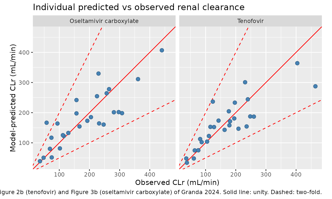
drug_cmp |>
  group_by(Drug) |>
  summarise(`R-squared (obs ~ pred)` =
              round(summary(lm(Observed ~ Reproduced))$adj.r.squared, 2),
            .groups = "drop") |>
  mutate(`Paper adjusted R-squared` = c(0.69, 0.71)) |>
knitr::kable(caption = "Goodness of fit vs the values displayed on Figure 2b / 3b.")| Drug | R-squared (obs ~ pred) | Paper adjusted R-squared |
|---|---|---|
| Oseltamivir carboxylate | 0.69 | 0.69 |
| Tenofovir | 0.71 | 0.71 |
The point of the paper: individualisation beats GFR alone
Granda 2024’s claim is that adding per-subject kidney blood flow and secretory capacity improves on a regression against measured GFR alone. Both comparators can be recomputed here.
comparator <- drug_cmp |>
  left_join(granda |> select(ID, iGFR), by = "ID") |>
  group_by(Drug) |>
  mutate(RegressionPred = fitted(lm(Observed ~ iGFR))) |>
  summarise(`Mechanistic mean error` = round(mean(abs(Reproduced - Observed)), 1),
            `iGFR regression mean error` = round(mean(abs(RegressionPred - Observed)), 1),
            .groups = "drop") |>
  mutate(`Paper mechanistic` = c(42.9, 37.1),
         `Paper regression`  = c(48.4, 41.7))
knitr::kable(comparator, caption = "Mean absolute prediction error (mL/min): mechanistic model vs linear regression on iGFR.")| Drug | Mechanistic mean error | iGFR regression mean error | Paper mechanistic | Paper regression |
|---|---|---|---|---|
| Oseltamivir carboxylate | 42.8 | 48.5 | 42.9 | 48.4 |
| Tenofovir | 37.0 | 41.8 | 37.1 | 41.7 |
The mechanistic model has the lower mean absolute error for both drugs, and both comparator values agree with the paper’s.
Assumptions and deviations
-
pka_acidis model-identified, not transcribed. Granda 2024 Table 2 lists molecular weight, LogP, unbound fraction, blood-to-plasma ratio and permeability but no pKa for any of the three compounds; neither do Huang & Isoherranen 2018 / 2020 nor Chang 2023 (which models tenofovir with the same kidney model). The value was therefore identified from the paper’s own tables rather than substituted from outside knowledge. Testing the two candidate readings against Tables 3 and 4 is decisive:Reading Kynurenic acid (Table 3) Tenofovir (Table 4) Oseltamivir carbox. (Table 4) Neutral / non-ionizing (framework sentinel pKa_a = 20)13/25 within 5%, median 0.951 median 0.979 median 0.915, 1/27 within 5% Fully ionized acid ( pKa_aat or below ~4.5)24/25 within 5%, median 1.005 median 1.001 median 1.005 The specific pKa is not identifiable: any
pka_acidat or below about 4.5 gives numerically identical predictions, because the un-ionized fraction is then below 0.1% across the tubular pH range 6.5-7.2 and every passive-diffusion term vanishes. The model-identified quantity is “un-ionized fraction is effectively zero”, not a chemical constant, andfixed(2)simply encodes that. No pKa was taken from an external database or assumed. fu_invitrois the framework default, not a Granda value. The intrinsic permeability ispapp / fu_invitro / 1.5. Granda 2024 does not report the un-ionized fraction in the transwell donor chamber, so the framework’s own distributed default of 1 is used (In_vitro_unionization = 1in the Huang & Isoherranen 2020 MATLAB code). This is provably immaterial here: because the compounds behave as fully ionized acids, the passive terms it scales are already negligible, and re-running the Table 3 reproduction atfu_invitro= 1, 0.5 and 0.2 gives identical results to four decimal places.CLint,secis the total across the three proximal-tubule subsegments. The model divides the tabulated value by 3 before applying it to each subsegment, and applies the same value to basolateral uptake and apical efflux (Granda 2024 Methods: “a range (10-1000 L/h) of secretory clearance values applied to both basolateral uptake and apical efflux clearance”). Two independent lines of evidence support the total-not-per-subsegment reading: back-solving the secretory clearance that reproduces each subject’s observed kynurenic acid clearance gives a ratio to the published value of 0.332-0.377 (median 0.357) across a 25-fold range ofCLint,sec; and Chang 2023 (Pharm Res, doi:10.1007/s11095-023-03594-x), which applies the same kidney model to tenofovir, writes its renal secretion as “30 L/hr (10 x 3)” – the total, with the per-subsegment value in parentheses.CLint,secis not re-scaled by kidney function. The back-solved ratio above shows no correlation with GFR, which spans 0.17 to 1.22 of healthy across this cohort; a GFR-proportional scaling would have produced a sevenfold spread. The tabulated value is used directly.Collecting-duct subsegment volume. Huang & Isoherranen 2018 Table 1 gives 0.237 L per collecting-duct subsegment; the 2020 distributed MATLAB code uses 0.009 L. The 2020 value is used here, because that is the code Granda actually ran. The choice is immaterial to every number in this vignette: steady-state
CLris identical to six significant figures under both, since compartment volumes affect only the approach to steady state and not the steady state itself.CRCLholds the raw, non-BSA-normalized iohexol clearance. Granda 2024 Table 3 tabulates absolute per-subject iohexol clearance in mL/min (cohort mean 90); Table 1 separately reports the BSA-normalized cohort summary of 76 +/- 30 mL/min/1.73 m^2. The mechanistic model needs the absolute whole-organ filtration flow, so the Table 3 column is the correct input. TheCRCLregister entry explicitly admits both normalized and raw forms and requires the per-model choice to be documented, whichcovariateData[[CRCL]]$descriptiondoes.KBFis a newly registered canonical covariate. Native kidney blood flow had no entry ininst/references/covariate-columns.md; the only flow-like renal entries (BFR,DFR,Q_CVVH,QBL,QEFF) are all extracorporeal-circuit quantities.KBFwas ratified alongside this extraction.No IIV and no residual error. Granda 2024 reports neither: the model is a deterministic per-subject forward predictor whose inputs are all measured or fitted per individual.
propSdis fixed at 0 rather than invented.The model files omit no reported mechanism, but the framework’s optional terms are inactive. Active apical and basolateral reabsorption and renal cellular metabolism are part of the Huang & Isoherranen framework and are kept in
ini()asfixed(0), matching the distributed MATLAB code, because none of these three compounds has a reported value for them. A user modelling a different compound can turn them on without editing the model body.