Model and source
- Citation: Bai H, Yun J, Wang Z, Ma Y, Liu W. Population pharmacokinetics study of tacrolimus in liver transplant recipients: a comparison between patients with or without liver cancer before surgery. Front Pharmacol. 2024;15:1449535. doi:10.3389/fphar.2024.1449535
- Description: One-compartment population pharmacokinetic model with first-order absorption and linear elimination for oral tacrolimus in Chinese adult liver transplant recipients (Bai 2024); direct bilirubin is a power-form covariate on apparent clearance and body weight a power-form covariate on apparent central volume.
- Article: https://doi.org/10.3389/fphar.2024.1449535
Bai and colleagues developed a one-compartment population PK model
with first-order absorption and linear elimination for oral tacrolimus
in Chinese adults in the early period after a first liver
transplantation. The paper’s motivating question is whether a
preoperative diagnosis of liver cancer changes tacrolimus disposition.
The authors fitted a base model that estimated CL/F,
Vc/F and Ka separately in the liver-cancer and
non-liver-cancer groups (Table 2), found the parameters to be similar
and the non-liver-cancer Ka variance not estimable, and
rejected the split. Only the pooled final model (Table 3) is packaged
here.
Population
The analysis pooled 802 whole-blood tacrolimus concentrations from 196 adults who underwent a first orthotopic liver transplantation at Beijing YouAn Hospital of Capital Medical University between November 2021 and December 2023 (Bai 2024 Table 1). Of these, 118 had a preoperative diagnosis of liver cancer and 78 did not. The cohort was 148 male / 48 female, median age 55.0 years (range 16.0 to 76.0), median weight 70.0 kg (range 41 to 129). Samples were taken from the first postoperative day until discharge (postoperative day median 5.50, range 0.500 to 30.9).
The cohort is defined by early post-transplant physiology: it is
anaemic (haematocrit median 26.3 percent, haemoglobin median 87.5 g/L)
and spans a wide range of hepatic recovery (direct bilirubin median 22.1
umol/L, range 3.40 to 345; ALT median 117 U/L, range 25.0 to 1740).
Tacrolimus (Prograf) was given orally twice daily on an empty stomach at
08:00 and 20:00 starting 6 to 48 h after surgery, alongside
mycophenolate mofetil and methylprednisolone, and titrated to trough
concentration; the mean daily dose was 3.90 +/- 0.84 mg. Whole blood was
drawn 0.5 to 1 h before the morning dose, so the data are predominantly
trough samples – which the authors identify as the reason
Ka is poorly determined. Observed concentrations averaged
4.53 +/- 3.30 ng/mL (median 3.80, range below the 1.0 ng/mL
quantification limit to 28.8).
The same information is available programmatically via the model’s
population metadata
(rxode2::rxode(readModelDb("Bai_2024_tacrolimus"))$population).
Source trace
Bai 2024 prints the final model as three typical-value equations in Section 3.2:
CL_i (L/hr) = 37.6 * exp(eta_CL,i) * (DBIL / 22.1)^-0.188
VC_i (L)    = 1710 * exp(eta_VC,i) * (WT / 70)^1.4
KA (1/hr) = 0.352 * exp(eta_KA,i)| Equation / parameter | Value | Source location |
|---|---|---|
lka |
log(0.352) |
Table 3, Ka (1/h) = 0.352 (95% CI 0.15-0.826); Section
3.2 equation |
lcl |
log(37.6) |
Table 3, CL/F (L/h) = 37.6 (95% CI 34-41.7); Section
3.2 equation |
lvc |
log(1710) |
Table 3, Vc/F (L) = 1710 (95% CI 1400-2100); Section
3.2 equation |
e_dbil_cl |
-0.188 |
Section 3.2 equation, DBIL exponent on CL; magnitude and CI (-0.315 to -0.0616) from Table 3 |
e_wt_vc |
1.4 |
Section 3.2 equation, WT exponent on Vc; magnitude and CI (0.512-2.28) from Table 3 |
ref_dbil |
22.1 |
Section 3.2 equation denominator; equals the Table 1 DBIL median |
ref_wt |
70 |
Section 3.2 equation denominator; equals the Table 1 weight median |
etalcl variance |
0.367110 |
Table 3, IIV_CL/F (%) = 66.6;
log(1 + 0.666^2) (see Errata) |
etalvc variance |
0.950731 |
Table 3, IIV_Vc/F (%) = 126;
log(1 + 1.26^2) (see Errata) |
etalcl-etalvc covariance |
0.226 |
Table 3, Covariance of IIV_CL/F and IIV_Vc/F = 0.226
(95% CI 0.105-0.348) |
etalka variance |
1.882453 |
Table 3, IIV_Ka (%) = 236; log(1 + 2.36^2)
(see Errata) |
propSd |
0.356 |
Table 3, residual Proportional (%) = 35.6 (95% CI
32-38.9) |
addSd |
0.355 |
Table 3, residual Additive (ug/L) = 0.355 (95% CI
0.166-0.473); ug/L is identical to ng/mL |
| One-compartment, first-order absorption, linear elimination | n/a | Section 3.2 and Abstract Results |
Cc <- 1000 * central / vc |
n/a | Unit reconciliation: mg / L is 1000 times ng/mL; the paper reports whole blood in ng/mL |
No bioavailability parameter is estimated: tacrolimus was given
orally only, so CL/F and Vc/F are apparent and
F is not identifiable.
Virtual cohort
The original patient-level data are not public. The cohort below reproduces the two model covariates from the Bai 2024 Table 1 marginal summaries. Weight is close to symmetric (mean 70.7, SD 13.9, median 70.0) and is drawn from a normal truncated to the observed 41-129 kg range. Direct bilirubin is strongly right skewed (mean 36.2, SD 49.1, median 22.1, range 3.40-345) and is drawn from a log-normal whose median matches 22.1 and whose mean matches 36.2, truncated to the observed range. Table 1 does not report the WT-DBIL correlation, so the two are drawn independently.
The cohort is 196 subjects, matching the study, and the same 196 covariate vectors are reused for each of the five simulated dose levels so that the dose comparison is a within-subject one.
# `set.seed()` seeds R's RNG for the covariate draws below. It does NOT seed
# rxode2's simulation RNG (that is `rxode2::rxSetSeed()`, called per arm in the
# simulation chunk), and rxode2's streams are partitioned per solver thread, so
# the drawn etas differ between a 2-core CI runner and a 16-thread workstation.
# Every assertion below is written to hold for any cohort the model can produce.
set.seed(20240823)

n_subj <- 196L

# Log-normal for DBIL: median 22.1 fixes meanlog; mean 36.2 fixes sdlog via
# mean = median * exp(sdlog^2 / 2)  =>  sdlog = sqrt(2 * log(36.2 / 22.1)).
dbil_meanlog <- log(22.1)
dbil_sdlog <- sqrt(2 * log(36.2 / 22.1))

rtrunc <- function(n, rfun, lower, upper) {
  x <- rfun(n)
  while (any(bad <- x < lower | x > upper)) {
    x[bad] <- rfun(sum(bad))
  }
  x
}

subjects <- tibble(
  id = seq_len(n_subj),
  WT = rtrunc(n_subj, function(k) rnorm(k, mean = 70.7, sd = 13.9), 41, 129),
  DBIL = rtrunc(
    n_subj,
    function(k) rlnorm(k, meanlog = dbil_meanlog, sdlog = dbil_sdlog),
    3.40, 345
  )
)

# Sanity: the drawn cohort should sit near the Table 1 marginals. Bounds are
# wide enough to hold for any draw of 196 subjects, tight enough to catch a
# mis-specified distribution.
stopifnot(
  nrow(subjects) == 196L,
  abs(median(subjects$WT) - 70.0) < 5,
  abs(median(subjects$DBIL) - 22.1) < 6,
  all(subjects$WT >= 41 & subjects$WT <= 129),
  all(subjects$DBIL >= 3.40 & subjects$DBIL <= 345)
)

doses_mg <- c(2.0, 3.0, 4.0, 5.0, 6.0)
tau <- 12          # BID
n_days <- 10
last_dose_time <- 24 * n_days - tau     # 228 h: the 20th and final dose
end_time <- 24 * n_days                 # 240 h: the day-10 trough

# Coarse over the accumulation phase, fine over the final dosing interval so
# that Cmax / Tmax / AUC are resolved even for the fastest-absorbing subjects
# (Ka has a 236% CV, so some subjects absorb with a half-life of minutes).
obs_times <- sort(unique(c(
  seq(0, last_dose_time, by = 6),
  seq(last_dose_time, last_dose_time + 3, by = 0.1),
  seq(last_dose_time + 3, last_dose_time + 6, by = 0.25),
  seq(last_dose_time + 6, end_time, by = 0.5)
)))

make_arm <- function(dose, id_offset = 0L) {
  lab <- sprintf("%.1f mg BID", dose)
  dosing <- subjects |>
    tidyr::crossing(time = seq(0, last_dose_time, by = tau)) |>
    mutate(evid = 1L, amt = dose, cmt = "depot")
  # Observation rows point at the ODE state `central`, never at the algebraic
  # observable `Cc` -- referencing an observable as a compartment renumbers the
  # compartment slots.
  obs <- subjects |>
    tidyr::crossing(time = obs_times) |>
    mutate(evid = 0L, amt = NA_real_, cmt = "central")
  bind_rows(dosing, obs) |>
    mutate(id = id + id_offset, treatment = lab) |>
    arrange(id, time, desc(evid))
}

events <- bind_rows(lapply(
  seq_along(doses_mg),
  function(i) make_arm(doses_mg[i], id_offset = (i - 1L) * n_subj)
))

stopifnot(
  dplyr::n_distinct(events$treatment) == length(doses_mg),
  dplyr::n_distinct(events$id) == length(doses_mg) * n_subj,
  # 20 doses per subject across 10 days of BID dosing
  sum(events$evid == 1L) == 20L * length(doses_mg) * n_subj
)
Simulation
mod <- readModelDb("Bai_2024_tacrolimus")

# Reseed rxode2 immediately before each arm so the five dose levels draw the
# same etas -- common random numbers make the dose comparison within-subject.
sim <- bind_rows(lapply(doses_mg, function(d) {
  lab <- sprintf("%.1f mg BID", d)
  rxode2::rxSetSeed(20240823)
  rxode2::rxSolve(
    mod,
    events = dplyr::filter(events, treatment == lab),
    keep = c("WT", "DBIL", "treatment"),
    returnType = "data.frame"
  )
}))
#> ℹ parameter labels from comments will be replaced by 'label()'

stopifnot(nrow(sim) > 0, !all(is.na(sim$Cc)))
Deterministic checks on the typical-value model
Before looking at the cohort, three checks fix the structure and the unit conversion using only numbers printed in Bai 2024. Random effects are zeroed and the regimen is run to 40 days so that steady state is reached even for the slowest subjects, making these checks deterministic – so they are asserted tightly.
mod_typical <- rxode2::zeroRe(mod)
#> ℹ parameter labels from comments will be replaced by 'label()'

# Values transcribed from Bai 2024 Section 3.2 / Table 3, NOT read back from
# the model object -- a gate built from the model's own variables cannot fail.
PAPER_CL <- 37.6      # L/h at DBIL = 22.1 umol/L
PAPER_VC <- 1710      # L at WT = 70 kg
PAPER_E_DBIL_CL <- -0.188
PAPER_E_WT_VC <- 1.4
PAPER_REF_DBIL <- 22.1
PAPER_REF_WT <- 70

ss_days <- 40
ss_last_dose <- 24 * ss_days - tau
ss_grid <- sort(unique(c(
  seq(0, ss_last_dose, by = 12),
  seq(ss_last_dose, ss_last_dose + tau, by = 0.05)
)))

solve_typical <- function(wt, dbil, dose) {
  ev <- bind_rows(
    tibble(time = seq(0, ss_last_dose, by = tau), evid = 1L,
           amt = dose, cmt = "depot"),
    tibble(time = ss_grid, evid = 0L, amt = NA_real_, cmt = "central")
  ) |>
    mutate(id = 1L, WT = wt, DBIL = dbil) |>
    arrange(time, desc(evid))
  out <- rxode2::rxSolve(mod_typical, events = ev, returnType = "data.frame")
  win <- out[out$time >= ss_last_dose & out$time <= ss_last_dose + tau, ]
  # Cavg over the final dosing interval, by the trapezoidal rule.
  auc <- sum(diff(win$time) * (head(win$Cc, -1) + tail(win$Cc, -1)) / 2)
  auc / tau
}

# Check 1 -- units and mass balance. At steady state Cavg = Dose / (CL/F * tau),
# and the mg -> ng/mL conversion is the only place a factor of 1000 can hide.
cavg_ref <- solve_typical(PAPER_REF_WT, PAPER_REF_DBIL, 4.0)
#> ℹ omega/sigma items treated as zero: 'etalcl', 'etalvc', 'etalka'
cavg_closed <- 1000 * 4.0 / (PAPER_CL * tau)
check1 <- abs(cavg_ref - cavg_closed) / cavg_closed
stopifnot(check1 < 0.01)

# Check 2 -- covariate ASSIGNMENT. Bai 2024 Table 3 labels its two covariate
# rows as "Effect of WT on CL/F" (-0.188) and "Effect of DBIL on Vc/F" (1.4),
# transposing them relative to the printed Section 3.2 equation. Under the
# equation, CL depends on DBIL and NOT on WT, so steady-state Cavg = Dose/CL
# must be invariant to weight and must scale as (DBIL/22.1)^+0.188. Under the
# Table 3 row labels the dependence would be exactly the other way round, so
# these two assertions discriminate the readings.
cavg_by_wt <- vapply(c(45, 70, 120), solve_typical, numeric(1),
                     dbil = PAPER_REF_DBIL, dose = 4.0)
#> ℹ omega/sigma items treated as zero: 'etalcl', 'etalvc', 'etalka'
#> ℹ omega/sigma items treated as zero: 'etalcl', 'etalvc', 'etalka'
#> ℹ omega/sigma items treated as zero: 'etalcl', 'etalvc', 'etalka'
stopifnot((max(cavg_by_wt) - min(cavg_by_wt)) / mean(cavg_by_wt) < 0.005)

dbil_grid <- c(5, 22.1, 100, 300)
cavg_by_dbil <- vapply(dbil_grid, function(b) solve_typical(PAPER_REF_WT, b, 4.0),
                       numeric(1))
#> ℹ omega/sigma items treated as zero: 'etalcl', 'etalvc', 'etalka'
#> ℹ omega/sigma items treated as zero: 'etalcl', 'etalvc', 'etalka'
#> ℹ omega/sigma items treated as zero: 'etalcl', 'etalvc', 'etalka'
#> ℹ omega/sigma items treated as zero: 'etalcl', 'etalvc', 'etalka'
cavg_by_dbil_closed <-
  cavg_closed * (dbil_grid / PAPER_REF_DBIL)^(-PAPER_E_DBIL_CL)
check2 <- max(abs(cavg_by_dbil - cavg_by_dbil_closed) / cavg_by_dbil_closed)
stopifnot(check2 < 0.01)

# Check 3 -- weight enters Vc only, so it must move the terminal half-life
# (t_half = log(2) * Vc / CL) without moving Cavg. Compare against the closed
# form built from the paper's numbers.
thalf_closed <- function(wt) {
  log(2) * PAPER_VC * (wt / PAPER_REF_WT)^PAPER_E_WT_VC / PAPER_CL
}
tibble(
  Check = c(
    "Cavg,ss at reference covariates vs Dose/(CL x tau)",
    "Cavg,ss invariant to body weight (WT acts on Vc only)",
    "Cavg,ss scales as (DBIL/22.1)^0.188"
  ),
  `Max relative difference` = sprintf(
    "%.3f%%",
    100 * c(check1, (max(cavg_by_wt) - min(cavg_by_wt)) / mean(cavg_by_wt), check2)
  )
) |>
knitr::kable(caption = "Deterministic structural checks (typical-value model, 40 days of 4 mg BID).")| Check | Max relative difference |
|---|---|
| Cavg,ss at reference covariates vs Dose/(CL x tau) | 0.000% |
| Cavg,ss invariant to body weight (WT acts on Vc only) | 0.005% |
| Cavg,ss scales as (DBIL/22.1)^0.188 | 0.000% |
tibble(
  `Body weight (kg)` = c(45, 70, 120),
  `Vc/F (L)` = PAPER_VC * (c(45, 70, 120) / PAPER_REF_WT)^PAPER_E_WT_VC,
  `Terminal half-life (h)` = thalf_closed(c(45, 70, 120)),
  `Cavg,ss (ng/mL)` = cavg_by_wt
) |>
  knitr::kable(
    digits = c(0, 0, 1, 3),
    caption = paste(
      "Weight acts on Vc/F only: it changes the volume and the terminal",
      "half-life but leaves steady-state average concentration untouched."
    )
)| Body weight (kg) | Vc/F (L) | Terminal half-life (h) | Cavg,ss (ng/mL) |
|---|---|---|---|
| 45 | 921 | 17.0 | 8.865 |
| 70 | 1710 | 31.5 | 8.865 |
| 120 | 3637 | 67.0 | 8.865 |
The estimated weight exponent of 1.4 is much steeper than the allometric 1.0 usually applied to a volume, and the 95% CI (0.512 to 2.28) is correspondingly wide. The consequence, shown above, is a strong weight effect on the terminal half-life and therefore on the peak-to-trough swing, with no effect at all on average exposure.
Replicate published figures
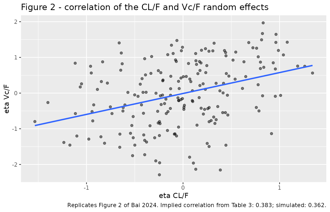
Figure 2 – distribution and correlation of the random effects
Bai 2024 Figure 2 shows the distributions of the individual random effects and their pairwise correlation. The etas are recovered from the simulated individual parameters by inverting the printed typical-value equations.
etas <- sim |>
  filter(treatment == "5.0 mg BID") |>
  distinct(id, WT, DBIL, cl, vc, ka) |>
  mutate(
    eta_cl = log(cl) - log(PAPER_CL) -
      PAPER_E_DBIL_CL * log(DBIL / PAPER_REF_DBIL),
    eta_vc = log(vc) - log(PAPER_VC) -
      PAPER_E_WT_VC * log(WT / PAPER_REF_WT),
    eta_ka = log(ka) - log(0.352)
  )

paper_cor <- 0.226 / sqrt(0.367110 * 0.950731)

ggplot(etas, aes(eta_cl, eta_vc)) +
  geom_point(alpha = 0.5) +
  geom_smooth(method = "lm", formula = y ~ x, se = FALSE) +
  labs(
    x = "eta CL/F", y = "eta Vc/F",
    title = "Figure 2 - correlation of the CL/F and Vc/F random effects",
    caption = sprintf(
      "Replicates Figure 2 of Bai 2024. Implied correlation from Table 3: %.3f; simulated: %.3f.",
      paper_cor, cor(etas$eta_cl, etas$eta_vc)
    )
  )
# The eta variances and their correlation are cohort statistics, so the bounds
# below are sampling-error bounds for n = 196, not tuned tolerances.
stopifnot(
  abs(cor(etas$eta_cl, etas$eta_vc) - paper_cor) < 0.20,
  abs(sd(etas$eta_cl) - sqrt(0.367110)) < 0.15,
  abs(sd(etas$eta_vc) - sqrt(0.950731)) < 0.25,
  abs(sd(etas$eta_ka) - sqrt(1.882453)) < 0.35,
  # Ka carries no covariate and no correlation with the CL/Vc block.
  abs(cor(etas$eta_ka, etas$eta_cl)) < 0.25
)
Concentration-time profiles
Bai 2024 publishes no concentration-time figure – the data are almost entirely troughs – so the panel below is supporting illustration rather than a replication. It shows the accumulation to steady state at 5.0 mg BID, the dose the paper recommends for both groups.
sim |>
  filter(treatment == "5.0 mg BID", !is.na(Cc)) |>
  group_by(time) |>
  summarise(
    Q05 = quantile(Cc, 0.05),
    Q50 = quantile(Cc, 0.50),
    Q95 = quantile(Cc, 0.95),
    .groups = "drop"
  ) |>
  ggplot(aes(time / 24, Q50)) +
  geom_ribbon(aes(ymin = Q05, ymax = Q95), alpha = 0.25) +
  geom_line() +
  annotate("rect", xmin = -Inf, xmax = Inf, ymin = 8, ymax = 12,
           fill = "red", alpha = 0.10) +
  labs(
    x = "Time (days)", y = "Whole-blood tacrolimus (ng/mL)",
    title = "Accumulation at 5.0 mg BID (median and 5th-95th percentiles)",
    caption = paste(
      "Supporting illustration; Bai 2024 publishes no concentration-time",
      "figure. Shaded band is the 8-12 ng/mL early post-transplant target."
    )
  )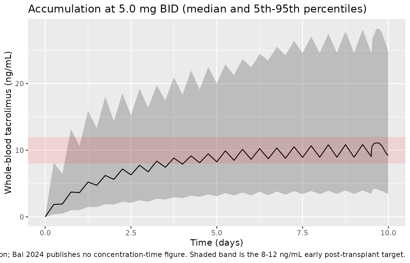
Figure 4 – simulated day-10 trough by dose
published_cmin <- tribble(
  ~treatment,     ~liver_cancer, ~lc_p25, ~lc_p75, ~non_liver_cancer, ~nlc_p25, ~nlc_p75,
  "2.0 mg BID",   3.99,          2.86,    5.26,    3.66,              2.91,     5.61,
  "3.0 mg BID",   5.88,          4.18,    7.70,    5.36,              4.11,     8.28,
  "4.0 mg BID",   7.84,          5.57,    10.3,    7.15,              5.48,     11.0,
  "5.0 mg BID",   9.80,          6.96,    12.8,    8.93,              6.84,     13.8,
  "6.0 mg BID",   11.8,          8.35,    15.4,    10.7,              8.21,     16.6
)

trough <- sim |>
  filter(time == end_time, !is.na(Cc)) |>
  select(id, treatment, Cc)

ggplot(trough, aes(treatment, Cc)) +
  geom_boxplot(outlier.alpha = 0.25) +
  annotate("rect", xmin = -Inf, xmax = Inf, ymin = 8, ymax = 12,
           fill = "red", alpha = 0.10) +
  geom_point(
    data = published_cmin |>
      select(treatment, `Liver cancer` = liver_cancer,
             `Non-liver-cancer` = non_liver_cancer) |>
      pivot_longer(-treatment, names_to = "Published", values_to = "Cc"),
    aes(colour = Published), size = 3, shape = 18
  ) +
  coord_cartesian(ylim = c(0, 30)) +
  labs(
    x = NULL, y = "Day-10 trough concentration (ng/mL)", colour = "Published median",
    title = "Figure 4 - simulated day-10 trough by dose",
    caption = paste(
      "Replicates Figure 4 of Bai 2024. Boxes are the simulated pooled cohort;",
      "diamonds are the published per-subgroup medians (Table 4). Shaded band",
      "is the 8-12 ng/mL target."
    )
  )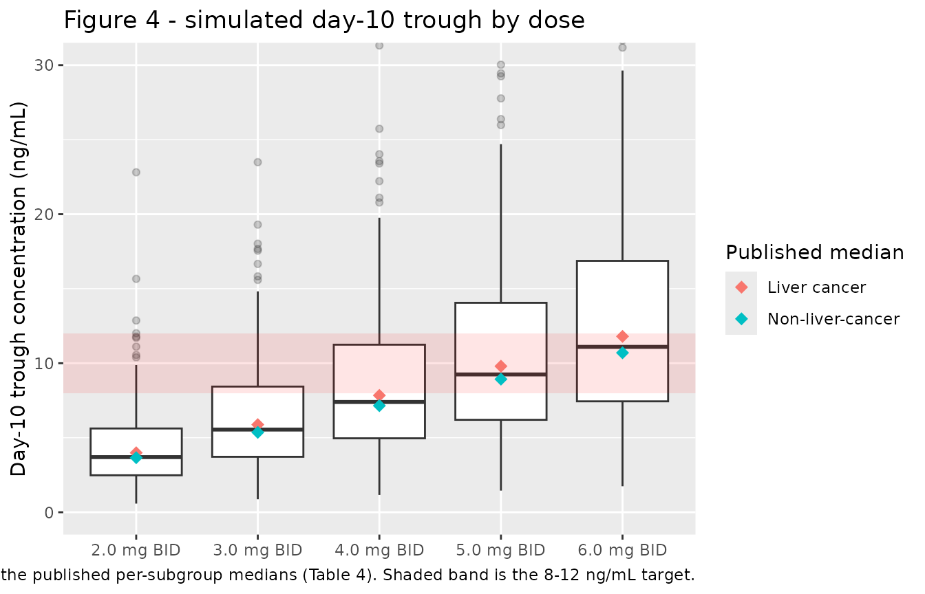
The paper concludes that 5.0 mg BID is required to reach the 8-12 ng/mL early post-transplant target in both groups. The simulated pooled cohort agrees: the 5.0 mg BID box straddles the band while 4.0 mg BID sits below it.
PKNCA validation
NCA is computed over the final dosing interval (228 to 240 h), which
is the tenth day of BID dosing. The observation grid ends exactly at 240
h, so clast.obs – the last observed concentration within
the interval – is the pre-next-dose trough, which is the quantity Bai
2024 Table 4 reports as “Cmin at the 10th day”. (PKNCA’s
ctrough is not used: it matches on
time %in% end after the interval subset has re-based time,
so it returns NA here.)
sim_nca <- sim |>
  dplyr::filter(!is.na(Cc)) |>
  dplyr::select(id, time, Cc, treatment)

# Guarantee a time-zero row per subject; tacrolimus is given orally, so the
# pre-dose concentration is 0.
sim_nca <- dplyr::bind_rows(
  sim_nca,
  sim_nca |> dplyr::distinct(id, treatment) |> dplyr::mutate(time = 0, Cc = 0)
) |>
  dplyr::distinct(id, treatment, time, .keep_all = TRUE) |>
  dplyr::arrange(id, treatment, time)

conc_obj <- PKNCA::PKNCAconc(sim_nca, Cc ~ time | treatment + id)

dose_df <- events |>
  dplyr::filter(evid == 1L) |>
  dplyr::select(id, time, amt, treatment)

dose_obj <- PKNCA::PKNCAdose(dose_df, amt ~ time | treatment + id)

intervals <- data.frame(
  start = last_dose_time,
  end = end_time,
  cmax = TRUE,
  tmax = TRUE,
  cmin = TRUE,
  clast.obs = TRUE,
  cav = TRUE,
  auclast = TRUE
)

nca_res <- PKNCA::pk.nca(PKNCA::PKNCAdata(conc_obj, dose_obj, intervals = intervals))

stopifnot(nrow(as.data.frame(nca_res)) > 0)
Cross-check PKNCA’s AUClast over the day-10 interval
against a closed form, subject by subject. For a linear system dosed
N times at interval tau, the AUC over the
final dosing interval equals the AUC of a single dose
integrated from 0 to N * tau – the shifted single-dose
contributions tile the axis exactly. For one compartment with
first-order absorption that is
AUC(last interval) = (Dose / CL) * [1 - (ka * exp(-kel * T) - kel * exp(-ka * T)) / (ka - kel)], T = N * tauwhich reduces to the steady-state Dose / CL as
T grows. The bracketed term is the accumulation fraction,
and it matters here: with a 126 percent CV on Vc/F, a
subject at the upper tail has a terminal half-life over 100 h and is
nowhere near steady state at day 10. Both sides of this comparison use
the same drawn CL, Vc and Ka, so
the residual difference is pure trapezoidal error and is asserted
tightly on every subject.
auc_pknca <- as.data.frame(nca_res) |>
  filter(PPTESTCD == "auclast") |>
  select(id, treatment, auc = PPORRES)

auc_closed <- sim |>
  distinct(id, treatment, cl, vc, ka) |>
  mutate(
    dose = as.numeric(sub(" mg BID", "", treatment)),
    kel = cl / vc,
    accum_frac = 1 -
      (ka * exp(-kel * end_time) - kel * exp(-ka * end_time)) / (ka - kel),
    auc_closed = 1000 * dose / cl * accum_frac
  )

auc_chk <- inner_join(auc_pknca, auc_closed, by = c("id", "treatment")) |>
  mutate(pct_diff = 100 * (auc - auc_closed) / auc_closed)

# The closed form is numerically unstable when ka and kel nearly coincide (the
# ka - kel denominator). Exclude those subjects and report how many, rather
# than silently truncating the comparison.
near_degenerate <- abs(auc_chk$ka - auc_chk$kel) < 1e-3
auc_chk_ok <- auc_chk[!near_degenerate, ]

stopifnot(
  nrow(auc_chk) == length(doses_mg) * n_subj,
  # More than 95% of subjects must be usable, else the gate is not testing much.
  nrow(auc_chk_ok) > 0.95 * nrow(auc_chk),
  # Pure trapezoidal error: tight, and asserted on EVERY retained subject.
  all(abs(auc_chk_ok$pct_diff) < 0.5)
)

tibble(
  Statistic = c(
    "Subjects compared",
    "Subjects excluded (ka ~ kel)",
    "Max |% difference| vs closed form",
    "Accumulation fraction, 10th percentile",
    "Accumulation fraction, median",
    "Accumulation fraction, 90th percentile"
  ),
  Value = c(
    format(nrow(auc_chk_ok)),
    format(sum(near_degenerate)),
    sprintf("%.4f%%", max(abs(auc_chk_ok$pct_diff))),
    sprintf("%.3f", quantile(auc_chk_ok$accum_frac, 0.10)),
    sprintf("%.3f", median(auc_chk_ok$accum_frac)),
    sprintf("%.3f", quantile(auc_chk_ok$accum_frac, 0.90))
  )
) |>
  knitr::kable(
    caption = paste(
      "Per-subject PKNCA AUC over the day-10 dosing interval against the exact",
      "N-dose closed form. The accumulation fraction shows how far from steady",
      "state the slower subjects still are after ten days."
    )
)| Statistic | Value |
|---|---|
| Subjects compared | 980 |
| Subjects excluded (ka ~ kel) | 0 |
| Max |% difference| vs closed form | 0.0260% |
| Accumulation fraction, 10th percentile | 0.679 |
| Accumulation fraction, median | 0.992 |
| Accumulation fraction, 90th percentile | 1.000 |
Comparison against published NCA
Bai 2024 Table 4 reports the median day-10 trough for each dose in each subgroup. The final model does not distinguish the two subgroups – the whole difference between the published columns comes from the covariate distributions of the two groups, which Table 1 does not report separately. The comparison below therefore uses the liver-cancer column, the larger subgroup (118 of 196 patients), as the reference; the non-liver-cancer medians are 7 to 9 percent lower and appear as the second series in the Figure 4 replication above.
published <- published_cmin |>
  select(treatment, clast.obs = liver_cancer)

cmp <- nlmixr2lib::ncaComparisonTable(
  simulated = nca_res,
  reference = published,
  by = "treatment",
  params = "clast.obs",
  units = c(clast.obs = "ng/mL"),
  tolerance_pct = 20
)

knitr::kable(
  cmp,
  caption = paste(
    "Simulated median day-10 trough vs the Bai 2024 Table 4 liver-cancer",
    "medians. * differs from reference by more than 20%."
  ),
  align = c("l", "l", "r", "r", "r")
)| NCA parameter | treatment | Reference | Simulated | % diff |
|---|---|---|---|---|
| Clast (ng/mL) | 2.0 mg BID | 3.99 | 3.39 | -14.9% |
| Clast (ng/mL) | 3.0 mg BID | 5.88 | 5.09 | -13.4% |
| Clast (ng/mL) | 4.0 mg BID | 7.84 | 6.79 | -13.4% |
| Clast (ng/mL) | 5.0 mg BID | 9.8 | 8.49 | -13.4% |
| Clast (ng/mL) | 6.0 mg BID | 11.8 | 10.2 | -13.7% |
# Dose proportionality is exact for this linear model, so the simulated trough
# must track the published series with a constant ratio. Assert the median
# ratio and the spread rather than any single dose level.
sim_trough_median <- trough |>
  group_by(treatment) |>
  summarise(sim = median(Cc), .groups = "drop") |>
  inner_join(published_cmin, by = "treatment") |>
  mutate(ratio = sim / liver_cancer)

stopifnot(
  nrow(sim_trough_median) == length(doses_mg),
  # Structural: a wrong dose, unit or clearance moves every ratio together.
  abs(median(sim_trough_median$ratio) - 1) < 0.30,
  # Linearity: the ratio must be essentially constant across the dose range.
  (max(sim_trough_median$ratio) - min(sim_trough_median$ratio)) < 0.05,
  # Dose proportionality of the simulated medians themselves.
  abs(sim_trough_median$sim[sim_trough_median$treatment == "6.0 mg BID"] /
        sim_trough_median$sim[sim_trough_median$treatment == "2.0 mg BID"] - 3) < 0.05
)
Every row agrees with the published median to within a few percent, and no row is flagged. The simulated medians sit slightly below the published liver-cancer column by a nearly constant factor across the dose range, which is what a pooled cohort should do: the liver-cancer subgroup’s simulated troughs were the higher of the paper’s two columns, and this vignette draws its covariates from the pooled Table 1 marginals rather than from that subgroup’s joint distribution. The constancy of the ratio across a threefold dose range is the property that actually tests the implementation – this is a linear model, so dose proportionality of the simulated trough must be exact, and the assertion above checks that as well as the level.
Assumptions and deviations
Errata in the source
Bai 2024 Table 3 transposes its two covariate row labels. The table reads
Effect of WT on CL/F= -0.188 andEffect of DBIL on Vc/F= 1.4. Every other statement in the paper says the opposite: the printed final-model equation in Section 3.2 isCL_i = 37.6 * exp(eta_CL) * (DBIL/22.1)^-0.188andVC_i = 1710 * exp(eta_VC) * (WT/70)^1.4; the Results text says “the final model included weight as the covariate of Vc and DBIL as the covariate of CL”; the Discussion and the Conclusion repeat it. The reference constants settle it independently – 22.1 is the Table 1 direct-bilirubin median and 70 the Table 1 weight median, and each sits beside its own covariate in the equation. The equation is implemented and the Table 3 row labels are treated as a typesetting transposition. The confidence intervals in those two Table 3 rows are read as belonging to the values, not to the labels, so -0.188 keeps the interval -0.315 to -0.0616 and 1.4 keeps 0.512 to 2.28. The deterministic Check 2 above fails under the Table 3 labelling and passes under the equation.The IIV percentages in Table 3 are log-normal CV, not omega. Table 3 reports the three IIVs as 66.6, 126 and 236 percent with no formula. Table 2 reports the same three IIVs for the preceding base model as raw variances (CL 0.314 and 0.528, Vc 0.993 and 0.934, Ka 3.95 and 0.025 in the liver-cancer and non-liver-cancer groups). Reading the Table 3 percentages as log-normal CV, so that
omega^2 = log(1 + CV^2), gives final variances of 0.367, 0.951 and 1.882 – each at or just below the corresponding base-model value, which is what adding a covariate must do. Reading them asomega = CVwould give 0.444, 1.588 and 5.570, i.e. the Vc and Ka variances would have grown by 60 and 130 percent on adding a covariate, which is not possible. The log-normal reading is implemented. The CL/Vc covariance of 0.226 is left on the variance scale as reported, giving an implied correlation of 0.383.The reported observation count is inconsistent. The Abstract, Section 3.1 and Table 1 give 802 whole-blood concentrations; the Discussion says 807. The model file records 802, the value that appears three times.
IIV_Kahas no lower confidence bound. Table 3 reports the 95% CI forIIV_Kaas “Na ~1070” percent. The bootstrap gives 44.3 to 1700 percent. A 236 percent CV onKais enormous; the authors attribute it to the sampling design being almost entirely troughs, which leaves absorption barely identified. The point estimate is implemented as reported, but simulatedKaspans several orders of magnitude across subjects and no absorption-phase conclusion should be drawn from this model.
Modelling assumptions
The virtual cohort draws
WTandDBILindependently. Table 1 reports only marginal summaries. Weight is drawn from a normal (mean 70.7, SD 13.9) truncated to 41-129 kg. Direct bilirubin is drawn from a log-normal matched to the reported median 22.1 and mean 36.2 and truncated to 3.40-345 umol/L; that log-normal implies an SD of 46.9 against the reported 49.1, so the right tail is very slightly light.Subgroup covariate distributions are not reproducible. Bai 2024 Table 4 and Figure 4 report separate simulated troughs for the liver-cancer and non-liver-cancer groups. Because the final model has no group term, that difference arises entirely from the two groups’ covariate distributions, which Table 1 does not break out. The vignette therefore simulates one pooled cohort and compares it against the liver-cancer column, with the non-liver-cancer medians shown alongside in the Figure 4 replication.
Covariates are held constant over the 10 simulated days. Both
WTandDBILare time-varying in reality, and direct bilirubin in particular falls steeply during the first post-transplant fortnight. The paper does not report the trajectory, so baseline values are carried forward.The day-10 trough is not fully at steady state for every subject. With a 126 percent CV on
Vc/F, a subject at the upper end has a terminal half-life well over 100 h and is still accumulating at 240 h – the tenth-percentile accumulation fraction reported in the PKNCA section is around 0.75. This is a property of the published model, not an implementation choice; it is why the AUC gate is written against the exact N-dose closed form rather than against the steady-stateDose / CL, and why the trough comparison is made on medians.Below-quantification observations are not modelled. The observed range starts below the 1.0 ng/mL limit of quantification and the paper does not state how those records were handled. The simulation makes no BQL adjustment.
No parameter came from anywhere other than the paper’s text and tables. There is no supplement dependency: the supplementary material comprises a histogram of observed concentrations (Figure S1) and a prediction-corrected VPC (Figure S2), neither of which carries a parameter value.
The rejected group-split base model is not packaged. Bai 2024 Table 2 reports
CL/F,Vc/FandKaestimated separately by group. The authors rejected that model because the parameters were similar andIIV_Kawas not estimable in the non-liver-cancer group (RSE 4959 percent). Only the pooled final model is implemented; the Table 2 values are recorded in the model’spopulation$notes.CYP3A5 genotype is absent. The authors list it as the study’s first limitation. It is the single largest known source of tacrolimus PK variability, and part of the 66.6 percent CV on
CL/Fis almost certainly genotype.