Piperacillin (Martinez-Casanova 2023)
Source:vignettes/articles/MartinezCasanova_2023_piperacillin.Rmd
MartinezCasanova_2023_piperacillin.RmdModel and source
Citation: Martinez-Casanova J, Esteve-Pitarch E, Colom-Codina H, Gumucio-Sanguino VD, Cobo-Sacristan S, Shaw E, Maisterra-Santos K, Sabater-Riera J, Perez-Fernandez XL, Rigo-Bonnin R, Tubau-Quintano F, Carratala J, Padulles-Zamora A (2023). Predictive Factors of Piperacillin Exposure and the Impact on Target Attainment after Continuous Infusion Administration to Critically Ill Patients. Antibiotics (Basel) 12(3):531. doi:10.3390/antibiotics12030531.
Description: Two-compartment population PK model for intravenous piperacillin (given as piperacillin-tazobactam by continuous infusion after a 4 g loading dose) in critically ill adults with preserved renal function (CKD-EPI eGFR >= 60 mL/min/1.73 m^2) (Martinez-Casanova 2023). First-order elimination from the central compartment, with clearance proportional to CKD-EPI estimated creatinine clearance centered at 99.24 mL/min/1.73 m^2. Between-subject variability on clearance only and a proportional residual error. Predicts TOTAL plasma piperacillin; tazobactam was not measured.
Article: https://doi.org/10.3390/antibiotics12030531 (open access, PMC10044067). The article has no supplement; the model is fully specified by Table 2 and its footnote. No erratum was found (Europe PMC, checked 2026-10-26).
Population
One hundred and six critically ill adults treated with piperacillin-tazobactam by continuous infusion in the intensive care unit of Bellvitge University Hospital, Barcelona, between August 2015 and June 2019 (Martinez-Casanova 2023 Methods 4.1, Table 1). Inclusion required preserved renal function – a CKD-EPI estimated creatinine clearance of at least 60 mL/min/1.73 m^2 – and excluded renal replacement therapy, extracorporeal membrane oxygenation, pregnancy and age under 18 years.
Median age 65 years (interquartile range 50-72), 67 % male, median weight 72 kg (65-84), median BMI 26.2 kg/m^2, 96 % Caucasian. Median CKD-EPI 97.1 mL/min/1.73 m^2 (86-114), with augmented renal clearance (CKD-EPI >= 130) in 11 patients. Median albumin 29 g/L; 34 % neurocritical, 35 % drainage carriers, 59 % mechanically ventilated and 42 % on vasoactive drugs.
Patients received a 4 g piperacillin (0.5 g tazobactam) loading dose over 30 min, then piperacillin 500 mg/h (12 g/day) by continuous infusion. Samples were drawn 30-60 min after the loading dose and at steady state (from 6 h after the infusion started): 218 total plasma concentrations, 2.1 per patient.
Source trace
| Model element | Value | Source |
|---|---|---|
| Structure: two compartments, first-order elimination from central | – | Results 2.2; Discussion |
lcl: CL at CKD-EPI 99.24 mL/min/1.73 m^2 |
12.0 L/h | Table 2, final model |
lvc: Vc |
20.7 L | Table 2 |
lvp: Vp |
62.4 L | Table 2 |
lq: CLD (intercompartmental clearance) |
4.77 L/h | Table 2 (abstract rounds to 4.8) |
CL covariate equation
TVCL = theta x (CRCL / 99.24)
|
linear, through origin | Table 2 footnote; Results 2.2 |
etalcl: omega^2 on CL (exponential) |
0.190 | Table 2; Methods 4.5.1 |
propSd: proportional residual SD |
sqrt(0.140) = 0.3742 | Table 2 (sigma^2 = 0.140); Results 2.2 |
| Unbound fraction for target attainment | fu = 0.7 | Methods 4.6 (30 % protein binding) |
| PTA scenarios: 8-24 g/day CI, CKD-EPI 60-200 in 20-unit bins, MIC 1-16 mg/L | – | Methods 4.6-4.7; Figure 4 |
Structural checks
The covariate equation and the continuous-infusion steady state are both deterministic for a typical patient, so they are checked to solver precision.
crcl_levels <- c(60, 99.24, 130, 200)
rate <- 500 # mg/h, the study regimen of 12 g/day

ev_ss <- rxode2::et(amt = 4000, dur = 0.5, cmt = "central") |>
  rxode2::et(time = 0.5, amt = rate * 400, dur = 400, cmt = "central") |>
  rxode2::et(c(0, 380, 400)) |>
  rxode2::et(id = seq_along(crcl_levels)) |>
  as.data.frame() |>
  dplyr::mutate(CRCL = crcl_levels[id])

typ <- rxode2::rxSolve(rxode2::zeroRe(mod), ev_ss, returnType = "data.frame") |>
  dplyr::filter(time == 380) |>
  dplyr::mutate(
    cl_expected = 12.0 * CRCL / 99.24,
    css_expected = rate / cl_expected
  )
#> ℹ omega/sigma items treated as zero: 'etalcl'
#> Warning: multi-subject simulation without without 'omega'

knitr::kable(
  typ |>
    dplyr::select(CRCL, cl, cl_expected, Cc, css_expected) |>
    dplyr::rename(
      "CKD-EPI (mL/min/1.73 m^2)" = CRCL,
      "Model CL (L/h)" = cl,
      "Table 2 CL (L/h)" = cl_expected,
      "Model Css (mg/L)" = Cc,
      "Rate / CL (mg/L)" = css_expected
    ),
  digits = 2,
  caption = "Typical clearance and steady-state concentration on 500 mg/h."
)| CKD-EPI (mL/min/1.73 m^2) | Model CL (L/h) | Table 2 CL (L/h) | Model Css (mg/L) | Rate / CL (mg/L) |
|---|---|---|---|---|
| 60.00 | 7.26 | 7.26 | 68.92 | 68.92 |
| 99.24 | 12.00 | 12.00 | 41.67 | 41.67 |
| 130.00 | 15.72 | 15.72 | 31.81 | 31.81 |
| 200.00 | 24.18 | 24.18 | 20.67 | 20.67 |
# Exact: a mis-transcribed CL, reference value or covariate form moves these
# by tens of percent. 380 h is about 20 terminal half-lives, so the residual
# approach-to-steady-state error is far below the tolerance.
stopifnot(
  max(abs(typ$cl / typ$cl_expected - 1)) < 1e-8,
  max(abs(typ$Cc / typ$css_expected - 1)) < 1e-4
)
The terminal half-life of the typical patient is long relative to the distribution volumes one might expect for a beta-lactam:
k10 <- 12.0 / 20.7
k12 <- 4.77 / 20.7
k21 <- 4.77 / 62.4
s <- k10 + k12 + k21
beta <- (s - sqrt(s^2 - 4 * k10 * k21)) / 2
alpha <- (s + sqrt(s^2 - 4 * k10 * k21)) / 2
c(alpha_half_life_h = log(2) / alpha, beta_half_life_h = log(2) / beta)
#> alpha_half_life_h  beta_half_life_h
#>         0.8316949        13.0359351
A 13 h terminal phase comes from the large, slowly equilibrating peripheral volume (62.4 L, estimated with 50.8 % RSE). In a continuous infusion the terminal phase only governs how fast the steady state is reached; the steady-state concentration itself is set by clearance alone.
Virtual cohort
CKD-EPI is drawn log-normally to match the Table 1 median and interquartile range (97.1, 86-114 mL/min/1.73 m^2) and truncated at the 60 mL/min/1.73 m^2 inclusion floor. Every patient receives the study regimen: 4 g over 30 min, then 500 mg/h.
# set.seed() seeds R's RNG (the CKD-EPI draw); rxSetSeed() seeds rxode2's
# simulation RNG, whose streams are partitioned per solver thread. The
# cohort therefore differs across machines and every assertion below is
# written on the centre of the distribution, not on its extremes.
set.seed(20230531)
rxode2::rxSetSeed(20230531)
n_sub <- 200

draw <- exp(rnorm(5 * n_sub, log(97.1), log(114 / 86) / (2 * qnorm(0.75))))
cohort <- data.frame(id = seq_len(n_sub), CRCL = draw[draw >= 60][seq_len(n_sub)])

obs_times <- sort(unique(c(0, 0.5, 0.75, 1, seq(2, 24, by = 2), seq(30, 300, by = 6))))
ev_cohort <- rxode2::et(amt = 4000, dur = 0.5, cmt = "central") |>
  rxode2::et(time = 0.5, amt = rate * 300, dur = 300, cmt = "central") |>
  rxode2::et(obs_times, cmt = "central") |>
  rxode2::et(id = cohort$id) |>
  as.data.frame() |>
  dplyr::left_join(cohort, by = "id")

sim <- rxode2::rxSolve(mod, ev_cohort, returnType = "data.frame") |>
  dplyr::mutate(treatment = "4 g LD + 12 g/day CI")

stopifnot(length(unique(sim$id)) == n_sub, all(cohort$CRCL >= 60))
quantile(cohort$CRCL, c(0.25, 0.5, 0.75))
#>       25%       50%       75%
#>  85.06596  99.93725 114.63361
Concentration-time profile (Figures 1 and 3)
vpc <- sim |>
  dplyr::group_by(time) |>
  dplyr::summarise(
    p05 = quantile(sim, 0.05),
    p50 = quantile(sim, 0.50),
    p95 = quantile(sim, 0.95),
    .groups = "drop"
  )

ggplot(vpc, aes(time)) +
  geom_ribbon(aes(ymin = p05, ymax = p95), fill = "steelblue", alpha = 0.3) +
  geom_line(aes(y = p50), colour = "firebrick") +
  labs(
    x = "Time from the start of the treatment (h)",
    y = "Total piperacillin (mg/L)"
  ) +
  theme_bw()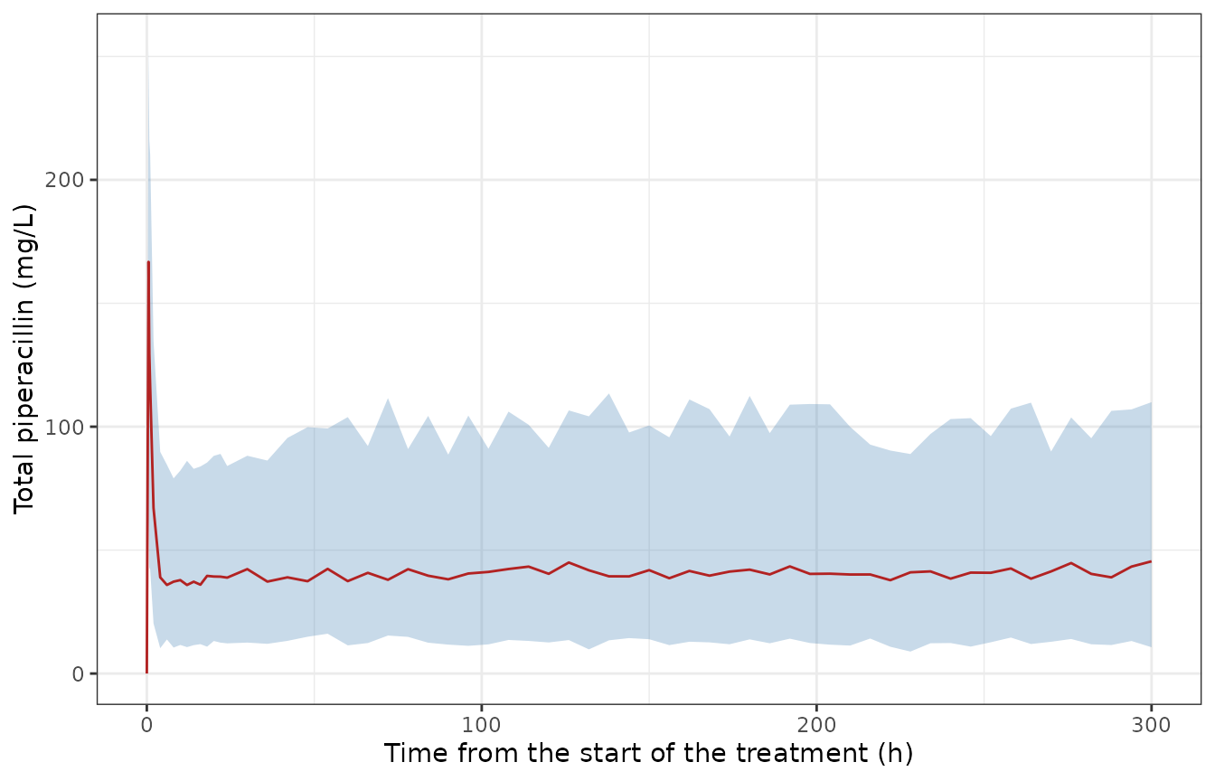
Simulated total piperacillin (5th, 50th and 95th percentiles of the prediction including residual error) over the axes of Figure 3 of Martinez-Casanova 2023 (prediction-corrected VPC; observed data are not public).
Figure 3 shows the observed median falling from roughly 150 mg/L shortly after the loading dose to a plateau near 40-50 mg/L from about 24 h, with the 97.5th percentile around 100-150 mg/L on the plateau. The simulated percentiles follow the same shape.
PKNCA validation
The paper reports two summary concentrations (Results 2.1): a geometric-mean “Cmax” of 112 mg/L, measured in samples drawn 30-60 min after the start of the loading dose, and a geometric-mean steady-state concentration Css of 39.5 mg/L, measured from 6 h after the start of the infusion. PKNCA computes Cmax over the first hour and the average concentration over the second day of the infusion for every simulated patient.
# Only !is.na(Cc): a time or concentration filter drops the time-zero row.
conc <- sim |>
  dplyr::filter(!is.na(Cc)) |>
  dplyr::select(id, time, Cc, treatment)

dose <- ev_cohort |>
  dplyr::filter(!is.na(amt), amt > 0) |>
  dplyr::select(id, time, amt) |>
  dplyr::mutate(treatment = "4 g LD + 12 g/day CI")

conc_obj <- PKNCA::PKNCAconc(conc, Cc ~ time | treatment + id)
dose_obj <- PKNCA::PKNCAdose(dose, amt ~ time | treatment + id)
intervals <- data.frame(
  start = c(0, 24),
  end = c(1, 48),
  cmax = c(TRUE, FALSE),
  cav = c(FALSE, TRUE)
)
nca <- PKNCA::pk.nca(PKNCA::PKNCAdata(conc_obj, dose_obj, intervals = intervals))
nca_res <- as.data.frame(nca)
summary(nca)
#>  start end            treatment   N       cmax         cav
#>      0   1 4 g LD + 12 g/day CI 200 158 [6.77]           .
#>     24  48 4 g LD + 12 g/day CI 200          . 41.1 [44.4]
#>
#> Caption: cmax, cav: geometric mean and geometric coefficient of variation; N: number of subjects
# The published values are geometric means; ncaComparisonTable() aggregates
# the simulated per-subject values by the median, which for a log-normal
# distribution is the geometric mean.
reference <- data.frame(
  treatment = "4 g LD + 12 g/day CI",
  cmax = 112,
  cav = 39.5
)
tbl <- nlmixr2lib::ncaComparisonTable(
  nca, reference,
  by = "treatment",
  units = c(cmax = "mg/L", cav = "mg/L")
)
knitr::kable(tbl, caption = "Simulated (median) versus published (geometric mean) concentrations, Results 2.1.")| NCA parameter | treatment | Reference | Simulated | % diff |
|---|---|---|---|---|
| Cmax (mg/L) | 4 g LD + 12 g/day CI | 112 | 160 | +42.7%* |
| Cavg (mg/L) | 4 g LD + 12 g/day CI | 39.5 | 41.9 | +6.1% |
if (!is.null(attr(tbl, "footnote"))) cat(attr(tbl, "footnote"), "\n")
#> * differs from reference by more than ±20%.
The simulated Cmax is the end-of-infusion peak at 0.5 h, whereas the published 112 mg/L comes from samples taken anywhere in the 30-60 min window, after the concentration has already started to fall in the distribution phase. The appropriate comparison for that sample is the geometric mean of the simulated concentrations across the sampling window:
gm <- function(x) exp(mean(log(x)))
window_gm <- sim |>
  dplyr::filter(time %in% c(0.5, 0.75, 1)) |>
  dplyr::group_by(time) |>
  dplyr::summarise(gm_Cc = gm(Cc), .groups = "drop")
knitr::kable(
  window_gm |> dplyr::rename("Time (h)" = time, "Geometric mean Cc (mg/L)" = gm_Cc),
  digits = 1
)| Time (h) | Geometric mean Cc (mg/L) |
|---|---|
| 0.5 | 157.5 |
| 0.8 | 132.9 |
| 1.0 | 113.2 |
cav_med <- nca_res |>
  dplyr::filter(PPTESTCD == "cav") |>
  dplyr::pull(PPORRES) |>
  median()

stopifnot(
  # The published geometric mean must lie within the simulated sampling
  # window: between the 1 h value and the 0.5 h value, with 15 % slack for
  # the unknown distribution of sampling times.
  window_gm$gm_Cc[window_gm$time == 1] < 112 * 1.15,
  window_gm$gm_Cc[window_gm$time == 0.5] > 112 * 0.85,
  # Central check on the steady-state concentration: a mis-transcribed CL,
  # reference CRCL or dose rate moves this by tens of percent.
  abs(cav_med / 39.5 - 1) < 0.20
)
The median day-2 average concentration is within about 10 % of the published geometric-mean Css. The observed Css samples were drawn from 6 h onwards, partly before the slow peripheral compartment had filled, and in patients whose dose was occasionally adjusted, so an exact match is not expected.
Probability of target attainment (Figure 4)
Methods 4.6 converts total to unbound concentration with fu = 0.7 and evaluates 100 % fT>1xMIC and 100 % fT>4xMIC at steady state for 8, 12, 16, 20 and 24 g/day by continuous infusion, CKD-EPI bins of 60-79 to 180-200 mL/min/1.73 m^2 and MICs of 1-16 mg/L.
During a continuous infusion at steady state the concentration is constant, so “100 % of the interval above the threshold” is simply Css >= threshold. The model carries between-patient variability on clearance only, so individual Css is the typical Css divided by exp(eta_CL). The probability of target attainment is therefore exact, with no Monte Carlo error:
PTA = Phi( log(fu x Css_typical / (k x MIC)) / omega_CL ).
The typical Css is taken from an rxode2 solve of the model. The formula rests on two facts about the model, both checked against a stochastic simulation before it is used: every simulated patient’s Css equals the infusion rate divided by that patient’s clearance, and log(CL_i / CL_typical) has standard deviation omega_CL.
rxode2::rxSetSeed(4)
ev_chk <- rxode2::et(amt = 4000, dur = 0.5, cmt = "central") |>
  rxode2::et(time = 0.5, amt = 16000 / 24 * 400, dur = 400, cmt = "central") |>
  rxode2::et(c(0, 380)) |>
  rxode2::et(id = 1:200) |>
  as.data.frame() |>
  dplyr::mutate(CRCL = 130)
chk <- rxode2::rxSolve(mod, ev_chk, returnType = "data.frame") |>
  dplyr::filter(time == 380)
cl_typ_chk <- 12.0 * 130 / 99.24
log_ratio <- log(chk$cl / cl_typ_chk)
c(sd_log_cl = sd(log_ratio), omega_cl = sqrt(0.190))
#> sd_log_cl  omega_cl
#> 0.4097913 0.4358899

stopifnot(
  nrow(chk) == 200,
  # Same drawn clearance on both sides, so the only difference is solver
  # error: a tight all() bound is correct here.
  max(abs(chk$Cc / ((16000 / 24) / chk$cl) - 1)) < 1e-4,
  # Sampling statistic of 200 draws: the SD of a log-normal sample of 200 has
  # a relative standard error of about 5 %, so 25 % is far outside noise but
  # catches a variance entered as an SD (or vice versa), which is a factor
  # of 2.3.
  abs(sd(log_ratio) / sqrt(0.190) - 1) < 0.25,
  abs(median(log_ratio)) < 0.15
)
omega_cl <- sqrt(ui$omega["etalcl", "etalcl"])
fu <- 0.7
bins <- data.frame(
  bin = c("60-79", "80-99", "100-119", "120-139", "140-159", "160-179", "180-200"),
  CRCL = seq(70, 190, by = 20)
)
doses <- c(8, 12, 16, 20, 24)

grid <- tidyr::expand_grid(bins, dose_g = doses)
# One typical patient per dose x bin: 4 g loading dose, then the daily dose as
# a continuous infusion (mg/h) for 400 h, observed at 380 h.
ids <- seq_len(nrow(grid))
ev_grid <- dplyr::bind_rows(
  data.frame(id = ids, time = 0, amt = 4000, dur = 0.5, evid = 1L),
  data.frame(id = ids, time = 0.5, amt = grid$dose_g * 1000 / 24 * 400, dur = 400, evid = 1L),
  data.frame(id = ids, time = 380, amt = NA_real_, dur = NA_real_, evid = 0L)
) |>
  dplyr::mutate(cmt = "central", CRCL = grid$CRCL[id]) |>
  dplyr::arrange(id, time)
css_typ <- rxode2::rxSolve(rxode2::zeroRe(mod), ev_grid, returnType = "data.frame") |>
  dplyr::filter(time == 380) |>
  dplyr::transmute(id, css = Cc)
#> ℹ omega/sigma items treated as zero: 'etalcl'
#> Warning: multi-subject simulation without without 'omega'

pta <- grid |>
  dplyr::mutate(id = dplyr::row_number()) |>
  dplyr::left_join(css_typ, by = "id") |>
  tidyr::expand_grid(mic = c(1, 4, 8, 16), k = c(1, 4)) |>
  dplyr::mutate(
    target = ifelse(k == 1, "100% fT>1xMIC", "100% fT>4xMIC"),
    pta = 100 * pnorm(log(fu * css / (k * mic)) / omega_cl),
    bin = factor(bin, levels = bins$bin)
  )
stopifnot(nrow(pta) == 7 * 5 * 4 * 2, !anyNA(pta$pta))
ggplot(pta, aes(bin, pta, colour = factor(dose_g), group = factor(dose_g))) +
  geom_line() +
  geom_point() +
  geom_hline(yintercept = 90, linetype = "dashed") +
  facet_grid(target ~ paste0("MIC = ", mic, " mg/L")) +
  labs(x = "CKD-EPI (mL/min/1.73 m^2)", y = "PTA (%)", colour = "g/24 h") +
  theme_bw() +
  theme(axis.text.x = element_text(angle = 90, vjust = 0.5, hjust = 1))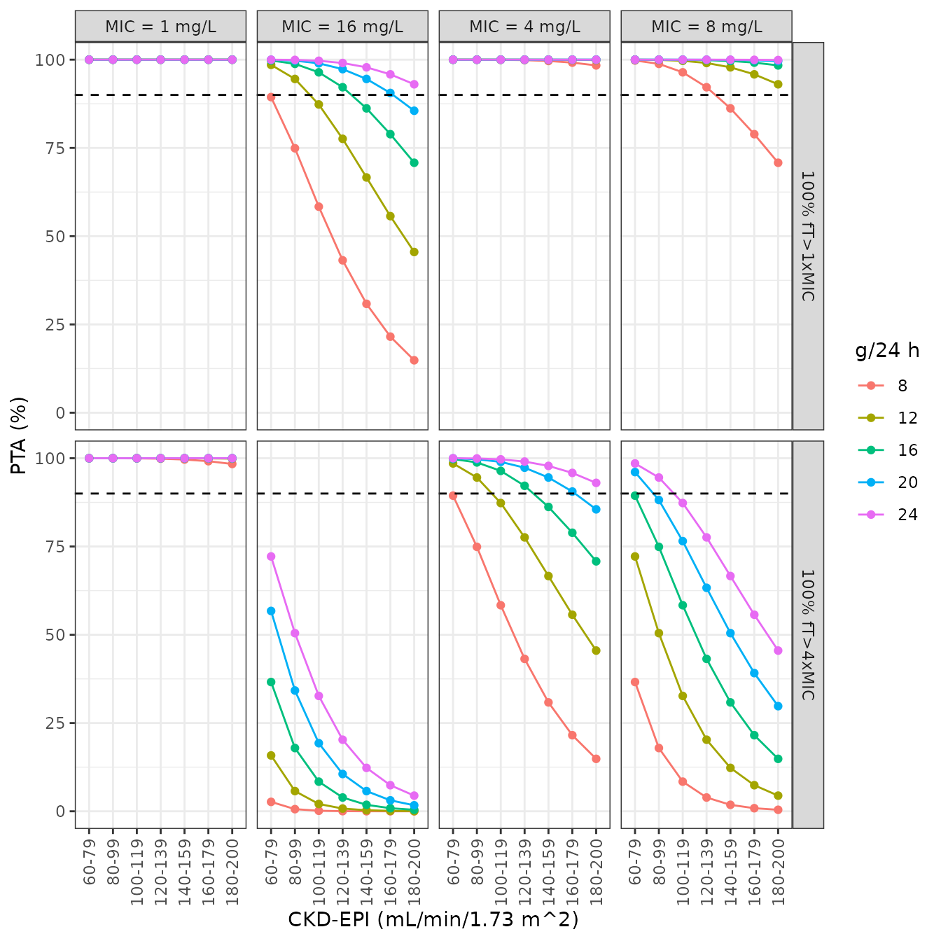
Replicates Figure 4 of Martinez-Casanova 2023: PTA at steady state by daily dose (g/24 h), CKD-EPI bin and MIC, for (top) 100 % fT>1xMIC and (bottom) 100 % fT>4xMIC. Dashed line: 90 % PTA.
Comparison with the published panels
The four panels of Figure 4 in which PTA varies (1xMIC at MIC 8 and 16 mg/L, 4xMIC at MIC 8 and 16 mg/L) were digitised by the maintainers, reading each marker to the nearest 0.5 percentage points. In the 1xMIC MIC 8 panel only the 8, 12 and 16 g lines separate from 100 %, so only those are compared.
fig4 <- list(
  "100% fT>1xMIC|8" = list(
    `8` = c(100, 98, 96, 91, 85, 78, 70),
    `12` = c(100, 100, 99.5, 98.5, 97, 94.5, 91.5),
    `16` = c(100, 100, 100, 99.5, 99, 98.5, 97)
  ),
  "100% fT>1xMIC|16" = list(
    `8` = c(91, 73.5, 58.5, 42.5, 30, 20.5, 14.5),
    `12` = c(98, 93, 86, 76.5, 65.5, 54.5, 44),
    `16` = c(100, 98.5, 95, 91, 85.5, 78.5, 70),
    `20` = c(100, 99.5, 98.5, 97, 94.5, 90, 84.5),
    `24` = c(100, 100, 99, 98.5, 97, 95, 92)
  ),
  "100% fT>4xMIC|8" = list(
    `8` = c(37, 16.5, 8, 4, 1.5, 0.5, 0),
    `12` = c(70.5, 48.5, 30.5, 19, 11.5, 7.5, 5),
    `16` = c(87, 74, 56.5, 42.5, 30.5, 21, 15),
    `20` = c(94.5, 87, 73.5, 63, 51, 39.5, 30.5),
    `24` = c(97, 93.5, 85, 76, 66, 55.5, 45.5)
  ),
  "100% fT>4xMIC|16" = list(
    `8` = c(1.5, 0.5, 0, 0, 0, 0, 0),
    `12` = c(11.5, 5, 1.5, 0.5, 0, 0, 0),
    `16` = c(28, 16, 6.5, 3, 1.5, 0.5, 0),
    `20` = c(47.5, 33, 15.5, 9.5, 5.5, 2.5, 1.5),
    `24` = c(62, 49, 27, 17.5, 11, 6.5, 3.5)
  )
)
published <- dplyr::bind_rows(lapply(names(fig4), function(panel) {
  parts <- strsplit(panel, "|", fixed = TRUE)[[1]]
  dplyr::bind_rows(lapply(names(fig4[[panel]]), function(d) {
    data.frame(
      target = parts[1], mic = as.numeric(parts[2]), dose_g = as.numeric(d),
      bin = bins$bin, pta_published = fig4[[panel]][[d]]
    )
  }))
}))

cmp <- published |>
  dplyr::mutate(bin = factor(bin, levels = bins$bin)) |>
  dplyr::inner_join(pta, by = c("target", "mic", "dose_g", "bin")) |>
  dplyr::mutate(diff = pta - pta_published)
# Guard against a silently empty or partial join.
stopifnot(nrow(cmp) == nrow(published), nrow(cmp) == 7 * 18)

cmp |>
  dplyr::group_by(target, mic) |>
  dplyr::summarise(
    cells = dplyr::n(),
    median_abs_diff = median(abs(diff)),
    max_abs_diff = max(abs(diff)),
    mean_signed_diff = mean(diff),
    .groups = "drop"
  ) |>
  dplyr::rename(
    "Target" = target, "MIC (mg/L)" = mic, "Cells" = cells,
    "Median |diff| (points)" = median_abs_diff,
    "Max |diff| (points)" = max_abs_diff,
    "Mean signed diff (points)" = mean_signed_diff
  ) |>
knitr::kable(digits = 1, caption = "Model PTA minus digitised Figure 4 PTA, percentage points.")| Target | MIC (mg/L) | Cells | Median |diff| (points) | Max |diff| (points) | Mean signed diff (points) |
|---|---|---|---|---|---|
| 100% fT>1xMIC | 8 | 21 | 0.6 | 1.5 | 0.6 |
| 100% fT>1xMIC | 16 | 35 | 0.7 | 1.6 | 0.6 |
| 100% fT>4xMIC | 8 | 35 | 0.7 | 3.0 | 0.8 |
| 100% fT>4xMIC | 16 | 35 | 0.7 | 10.2 | 1.8 |
cmp |>
  dplyr::filter(target == "100% fT>1xMIC", mic == 16) |>
  dplyr::mutate(cell = sprintf("%.1f (%.1f)", pta, pta_published)) |>
  dplyr::select(dose_g, bin, cell) |>
  tidyr::pivot_wider(names_from = bin, values_from = cell) |>
  dplyr::rename("Dose (g/24 h)" = dose_g) |>
knitr::kable(caption = "100 % fT>1xMIC at MIC 16 mg/L: model PTA (digitised Figure 4 PTA), %.")| Dose (g/24 h) | 60-79 | 80-99 | 100-119 | 120-139 | 140-159 | 160-179 | 180-200 |
|---|---|---|---|---|---|---|---|
| 8 | 89.4 (91.0) | 74.9 (73.5) | 58.4 (58.5) | 43.2 (42.5) | 30.8 (30.0) | 21.5 (20.5) | 14.9 (14.5) |
| 12 | 98.5 (98.0) | 94.5 (93.0) | 87.3 (86.0) | 77.6 (76.5) | 66.6 (65.5) | 55.7 (54.5) | 45.5 (44.0) |
| 16 | 99.8 (100.0) | 98.8 (98.5) | 96.4 (95.0) | 92.2 (91.0) | 86.2 (85.5) | 78.9 (78.5) | 70.8 (70.0) |
| 20 | 100.0 (100.0) | 99.7 (99.5) | 99.0 (98.5) | 97.3 (97.0) | 94.5 (94.5) | 90.6 (90.0) | 85.5 (84.5) |
| 24 | 100.0 (100.0) | 99.9 (100.0) | 99.7 (99.0) | 99.1 (98.5) | 97.8 (97.0) | 95.8 (95.0) | 93.0 (92.0) |
# Both sides are deterministic (an exact formula and a fixed digitisation),
# so these bounds do not depend on the machine or the rxode2 build. They sit
# above digitisation error (about 1 point) and the internal inconsistency of
# the published 4xMIC, MIC 16 panel (see below), but a halved dose rate, a
# dropped covariate term or a mis-scaled omega moves whole panels by 10-40
# points.
stopifnot(
  median(abs(cmp$diff)) < 2,
  quantile(abs(cmp$diff), 0.9) < 6,
  abs(mean(cmp$diff)) < 2
)
The model reproduces Figure 4 to within digitisation error almost everywhere. The largest differences are in the 60-79 mL/min/1.73 m^2 bin of the 4xMIC, MIC 16 mg/L panel, where the model is up to about 10 points higher than the published curve for the 16-24 g doses. That panel is inconsistent with the rest of the published figure: because steady-state PTA depends only on dose / (k x MIC), 4xMIC at MIC 16 mg/L on dose D must equal 4xMIC at MIC 8 mg/L on dose D/2, and the published figure gives 28 % (16 g, MIC 16) against 37 % (8 g, MIC 8) and 62 % (24 g, MIC 16) against 70.5 % (12 g, MIC 8) for the same bin. The model matches the MIC 8 mg/L panel there, so the residual reflects the published simulation (Monte Carlo noise or a different CKD-EPI sampling within that bin) rather than the parameters.
The paper’s conclusions follow from these curves: on 12 g/day the 1xMIC target exceeds 90 % for MICs up to 8 mg/L in every bin, while at MIC 16 mg/L 12 g/day falls below 90 % from the 100-119 bin onwards and 16 g/day from the 140-159 bin onwards.
Assumptions and deviations
- Covariate reference value. The Table 2 footnote centres CL at 99.24 mL/min/1.73 m^2, while Table 1 reports a cohort median of 97.1. The printed equation is used; the paper does not say which records 99.24 is the median of (possibly all sampling occasions rather than baseline).
- Time-varying CKD-EPI. Covariates were recorded at baseline and on each sampling occasion, but the paper does not say whether CKD-EPI entered the final model as time-varying. The model accepts either; the simulations here hold it constant per patient.
- Residual error. Table 2 reports the NONMEM variance sigma^2 = 0.140 of a proportional error model; the model stores the SD, sqrt(0.140) = 0.3742.
- CKD-EPI within a bin. The PTA replication evaluates each 20-unit bin at its midpoint (70, 90, …, 190 mL/min/1.73 m^2). The paper does not say how CKD-EPI was sampled within a bin.
- Steady state in the PTA. Figure 4 is described as PTA “at steady state”; with a continuous infusion that is Css >= k x MIC / fu, evaluated exactly from the model rather than by Monte Carlo. Residual error is not added, since target attainment concerns the true concentration.
- Cumulative fraction of response (Table 3) is not reproduced. It weights PTA by the 2023 EUCAST wild-type MIC distribution of Pseudomonas aeruginosa, which the paper cites but does not print.
- Virtual cohort. CKD-EPI is log-normal with the Table 1 median and interquartile range, truncated at 60 mL/min/1.73 m^2. Other demographics do not enter the model. The study’s occasional dose adjustments (four occasions, three patients) and the patients who skipped the loading dose are not simulated.
- Unbound concentrations. The model predicts total plasma piperacillin. Unbound concentration is 0.7 x Cc, following the paper’s assumed 30 % protein binding. Tazobactam was not measured and is not modelled.