Candesartan (Kassem 2021)
Source:vignettes/articles/Kassem_2021_candesartan.Rmd
Kassem_2021_candesartan.RmdModel and source
- Citation: Kassem I, Sanche S, Li J, Bonnefois G, Dube MP, Rouleau JL, Tardif JC, White M, Turgeon J, Nekka F, de Denus S. Population pharmacokinetics of candesartan in patients with chronic heart failure. Clin Transl Sci. 2021 Jan;14(1):194-203. doi:10.1111/cts.12842. PMCID: PMC7877833.
- Description: One-compartment population PK model for oral candesartan (dosed as the prodrug candesartan cilexetil) in white adults with chronic heart failure and reduced ejection fraction (Kassem 2021). First-order absorption with a lag time feeds a one-compartment disposition model. Apparent clearance carries median-normalised power effects of body weight and eGFR and a multiplicative effect of diabetes; interindividual variability is estimated on apparent clearance only. Combined additive + proportional residual error.
- Article: https://doi.org/10.1111/cts.12842
Candesartan is an angiotensin II receptor blocker given orally as the prodrug candesartan cilexetil, which is completely hydrolysed to candesartan during absorption. Kassem 2021 characterised candesartan population PK in patients with chronic heart failure (HF) with reduced ejection fraction who were titrated from 4 mg to a 32 mg once-daily target, and identified body weight, estimated glomerular filtration rate (eGFR) and diabetes as determinants of apparent oral clearance (CL/F).
Population
The analysis used 1,455 plasma concentrations from 281 white patients enrolled at 16 Canadian centres in a prospective, open-label pharmacogenomic study (Results; Table 1). Patients had symptomatic HF with left ventricular ejection fraction at most 40% (mean 29.2%) and NYHA class II (78.3%) or III-IV (21.7%). Mean (SD) age was 65.6 (10.0) years and weight 84.0 (19.1) kg; 17% were women. Mean eGFR was 74.2 (22.3) mL/min/1.73 m^2, and 32.7% had diabetes. The candesartan cilexetil dose was escalated at each titration visit (4, 8, 16 and 32 mg once daily) when tolerated. The first sample was drawn 2 h after the first 4 mg dose; later samples were taken at whatever time after the previous dose the visit fell, and most were within 0-4 h post-dose (Figure S2).
The same information is available programmatically via
readModelDb("Kassem_2021_candesartan")()$population.
Source trace
Every value comes from Table 2 (final model) and the final-model CL/F
equation in Results; the in-file comments in
inst/modeldb/specificDrugs/Kassem_2021_candesartan.R carry
the same trace.
| Equation / parameter | Value | Source location |
|---|---|---|
lcl (CL/F, non-diabetic, 82.45 kg, eGFR 74) |
8.63 L/h (RSE 4%) | Table 2, CL/F - theta1
|
lvc (Vd/F) |
12.5 L (RSE 10%) | Table 2, Vd/F - theta2
|
lka |
0.131 1/h (RSE 6%) | Table 2, Ka - theta3
|
ltlag |
0.165 h (RSE 3%) | Table 2, TLAG - theta4
|
e_wt_cl |
0.963 (RSE 15%) | Table 2, Weight effect on CL/F - theta5
|
e_crcl_cl |
0.56 (RSE 18%) | Table 2, eGFR effect on CL/F - theta6
|
e_diab_cl |
0.682 (RSE 8%) | Table 2, Diabetes effect on CL/F - theta7
|
etalcl |
variance 0.138 (RSE 7%) | Table 2, omega2 CL/F
|
addSd |
sqrt(5.5) = 2.345 ng/mL | Table 2, sigma2 (additive) = 5.5 |
propSd |
sqrt(0.418) = 0.6465 | Table 2, sigma2 (proportional) = 0.418 |
| CL/F = 8.63 (WT/82.45)^0.963 (eGFR/74)^0.56 0.682^Diabetes exp(eta) | n/a | Results, final-model equation |
| Reference weight 82.45 kg, eGFR 74 | n/a | Table 2 footnote (cohort medians) |
| Diabetes coding 0 = no, 1 = yes | n/a | Supplementary Table S1 footnote |
| One compartment, first-order absorption, lag, mixed error, diagonal omega | n/a | Results, model-development paragraph |
Bootstrap means and 95% CIs (Table 3) contain every Table 2 estimate.
Structural checks
mod <- rxode2::rxode(readModelDb("Kassem_2021_candesartan"))

# The explicit d/dt() system must be solved as written, not auto-replaced by a
# closed-form linear compartment solution.
stopifnot(is.null(mod$linCmt))

typ_grid <- seq(0.05, 120, by = 0.05)
typ_events <- data.frame(
  id = 1L,
  time = c(0, typ_grid),
  amt = c(4, rep(NA_real_, length(typ_grid))),
  evid = c(1L, rep(0L, length(typ_grid))),
  cmt = c("depot", rep("central", length(typ_grid))),
  WT = 82.45,
  CRCL = 74,
  DIS_DIAB = 0L
)

typ <- rxode2::rxSolve(rxode2::zeroRe(mod), events = typ_events, omega = NA) |>
  as.data.frame()

cl_typ <- unique(round(typ$cl, 6))
vc_typ <- unique(round(typ$vc, 6))
tmax_typ <- typ$time[which.max(typ$Cc)]
c2h_typ <- typ$Cc[abs(typ$time - 2) < 1e-8]

round(c(
  CL_L_per_h = cl_typ, V_L = vc_typ, tmax_h = tmax_typ,
  Cmax_ng_per_mL = max(typ$Cc), C2h_ng_per_mL = c2h_typ
), 3)
#>     CL_L_per_h            V_L         tmax_h Cmax_ng_per_mL  C2h_ng_per_mL
#>          8.630         12.500          3.150         41.141         37.815
With ka = 0.131 1/h and kel = CL/V = 0.69 1/h the model is flip-flop: the terminal slope is set by absorption, so the terminal half-life of a typical patient is ln(2)/ka = 5.3 h and the typical peak falls about 3.2 h after the dose – consistent with the 3-4 h tmax usually reported for candesartan.
# Check 1 -- the typical CL/F and V/F are the Table 2 values.
stopifnot(abs(cl_typ - 8.63) < 1e-4, abs(vc_typ - 12.5) < 1e-4)

# Check 2 -- dose recovery. F is absorbed into CL/F and V/F, so
# CL/F * AUC(0-inf) must return the 4 mg dose (AUC in ng.h/mL -> mg.h/L).
auc_trap <- sum(diff(c(0, typ$time)) * (c(0, utils::head(typ$Cc, -1)) + typ$Cc) / 2)
lz <- -diff(log(utils::tail(typ$Cc, 2))) / 0.05
auc_inf <- (auc_trap + utils::tail(typ$Cc, 1) / lz) / 1000
stopifnot(
  abs(cl_typ * auc_inf / 4 - 1) < 0.005,
  # Mutation control: a 20% wrong clearance must not recover the dose.
  abs(cl_typ * 1.2 * auc_inf / 4 - 1) > 0.05,
  # Terminal slope is the absorption rate constant (flip-flop).
  abs(lz - 0.131) < 0.001
)
round(c(auc_inf_mg_h_per_L = auc_inf, dose_recovered_mg = cl_typ * auc_inf), 3)
#> auc_inf_mg_h_per_L  dose_recovered_mg
#>              0.464              4.000
Figure 3: covariate effects on CL/F
Figure 3 of Kassem 2021 gives, for single covariate values, the
probability that CL/F falls more than 25% below the population typical
value. Those probabilities are reproduced to within one percentage point
when the covariate effect is drawn from the parameter
uncertainty (normal, SE = RSE x estimate from Table 2)
rather than from interindividual variability. For a power effect
(x/ref)^theta the event “CL/F ratio < 0.75” is
theta > log(0.75)/log(x/ref) when
x < ref; for the diabetes factor it is
theta7 < 0.75.
th <- c(wt = 0.963, gfr = 0.56, diab = 0.682)
se <- c(wt = 0.15 * 0.963, gfr = 0.18 * 0.56, diab = 0.08 * 0.682)

p_power_drop <- function(x, ref, est, sd) {
  1 - stats::pnorm(log(0.75) / log(x / ref), mean = est, sd = sd)
}

fig3 <- tibble::tribble(
  ~scenario, ~typical_ratio, ~p_drop_gt25, ~published,
  "Diabetes",
  th[["diab"]], stats::pnorm(0.75, th[["diab"]], se[["diab"]]), 0.90,
  "Weight = 60 kg",
  (60 / 82.45)^th[["wt"]], p_power_drop(60, 82.45, th[["wt"]], se[["wt"]]), 0.65,
  "eGFR = 45",
  (45 / 74)^th[["gfr"]], p_power_drop(45, 74, th[["gfr"]], se[["gfr"]]), 0.42
)

fig3 |>
  mutate(
    typical_change_pct = 100 * (typical_ratio - 1),
    p_drop_gt25 = 100 * p_drop_gt25,
    published = 100 * published
  ) |>
  select(scenario, typical_change_pct, p_drop_gt25, published) |>
  dplyr::rename(
    "Scenario" = scenario,
    "Typical CL/F change (%)" = typical_change_pct,
    "P(decrease > 25%), model (%)" = p_drop_gt25,
    "P(decrease > 25%), Figure 3 (%)" = published
  ) |>
knitr::kable(digits = 1, caption = "Replicates the single-covariate probabilities of Figure 3 of Kassem 2021.")| Scenario | Typical CL/F change (%) | P(decrease > 25%), model (%) | P(decrease > 25%), Figure 3 (%) |
|---|---|---|---|
| Diabetes | -31.8 | 89.4 | 90 |
| Weight = 60 kg | -26.4 | 65.6 | 65 |
| eGFR = 45 | -24.3 | 42.8 | 42 |
# Deterministic gate: every probability within 2 percentage points.
stopifnot(all(abs(fig3$p_drop_gt25 - fig3$published) < 0.02))

# Mutation control: the same probability for diabetes computed from the IIV
# (omega2 = 0.138) instead of parameter uncertainty is about 60%, far from the
# published 90%, so the gate discriminates between the two readings.
p_iiv <- stats::pnorm((log(0.75) - log(0.682)) / sqrt(0.138))
stopifnot(abs(p_iiv - 0.90) > 0.2)
round(p_iiv, 3)
#> [1] 0.601
This confirms the transcription of the three covariate coefficients, the two normalising medians (82.45 kg and 74 mL/min/1.73 m^2) and the power / multiplicative forms together.
Virtual cohort
Observed data are not public. The cohort draws weight and eGFR independently from normal distributions with the Table 1 means and SDs, and diabetes as a Bernoulli variable with the Table 1 prevalence. Weight and eGFR outside plausible ranges are rejected and redrawn (not clamped).
set.seed(20210101)
n_sub <- 200L

draw_trunc <- function(n, mean, sd, lo, hi) {
  out <- numeric(0)
  while (length(out) < n) {
    x <- stats::rnorm(n, mean, sd)
    out <- c(out, x[x >= lo & x <= hi])
  }
  out[seq_len(n)]
}

subjects <- tibble(
  id = seq_len(n_sub),
  WT = draw_trunc(n_sub, 84.0, 19.1, 40, 160),
  CRCL = draw_trunc(n_sub, 74.2, 22.3, 15, 150),
  DIS_DIAB = stats::rbinom(n_sub, 1, 0.327)
) |>
  mutate(
    # Kassem 2021 'predicted low-clearance population' (Table 4 footnote).
    low_cl = (DIS_DIAB == 1 & CRCL <= 60) | (WT <= 70 & CRCL <= 45)
  )

round(c(
  WT_mean = mean(subjects$WT), CRCL_mean = mean(subjects$CRCL),
  diabetes_pct = 100 * mean(subjects$DIS_DIAB),
  low_cl_pct = 100 * mean(subjects$low_cl)
), 1)
#>      WT_mean    CRCL_mean diabetes_pct   low_cl_pct
#>         85.9         74.2         33.0         11.0
Table 4: concentration 2 h after the first 4 mg dose
At week 0 every patient received 4 mg candesartan cilexetil and was sampled 2 h later. Table 4 reports a mean (SD) of 44 (34) ng/mL in 208 patients outside the predicted low-clearance group and 52 (33.3) ng/mL in 38 inside it. The simulation below includes residual error, since the table summarises observations.
ev_2h <- bind_rows(
  subjects |> mutate(time = 0, amt = 4, evid = 1L, cmt = "depot"),
  subjects |> mutate(time = 2, amt = NA_real_, evid = 0L, cmt = "central")
) |>
  arrange(id, time, desc(evid))

rxode2::rxSetSeed(20210102)
sim_2h <- rxode2::rxSolve(
  mod,
  events = ev_2h,
  omega = mod$omega,
  keep = c("low_cl"),
  addDosing = FALSE
) |>
  as.data.frame()

stopifnot(dplyr::n_distinct(round(sim_2h$cl, 8)) > 1L)

tab4 <- sim_2h |>
  group_by(low_cl) |>
  summarise(n = dplyr::n(), mean_sim = mean(sim), sd_sim = sd(sim), .groups = "drop") |>
  mutate(
    mean_obs = ifelse(low_cl, 52, 44),
    sd_obs = ifelse(low_cl, 33.3, 34)
  )

tab4 |>
  dplyr::rename(
    "Predicted low clearance" = low_cl,
    "N simulated" = n,
    "Simulated mean (ng/mL)" = mean_sim,
    "Simulated SD (ng/mL)" = sd_sim,
    "Table 4 mean (ng/mL)" = mean_obs,
    "Table 4 SD (ng/mL)" = sd_obs
  ) |>
knitr::kable(digits = 1, caption = "Replicates the week-0 rows of Table 4 of Kassem 2021.")| Predicted low clearance | N simulated | Simulated mean (ng/mL) | Simulated SD (ng/mL) | Table 4 mean (ng/mL) | Table 4 SD (ng/mL) |
|---|---|---|---|---|---|
| FALSE | 178 | 38.7 | 27.0 | 44 | 34.0 |
| TRUE | 22 | 45.0 | 28.9 | 52 | 33.3 |
# Pooled centre: Table 4 week-0 pooled mean is (208 * 44 + 38 * 52) / 246 = 45.2.
# The centre is gated on the residual-free individual prediction (`ipredSim`):
# the proportional error is mean-zero, so it moves the expected mean not at all
# but adds most of the sampling noise, and dropping it keeps the gate stable
# across random-number streams.
pooled_obs <- (208 * 44 + 38 * 52) / 246
pooled_sd_obs <- 34
mean_ipred <- mean(sim_2h$ipredSim)

# Alternative readings, each checked against the same observations:
# (a) doses in candesartan free-acid equivalents (x 440.5 / 610.7);
mw_ratio <- 440.5 / 610.7
# (b) the Table 2 proportional sigma read as an SD rather than a variance.
mod_sd_reading <- suppressMessages(mod |> rxode2::ini(propSd = 0.418))
rxode2::rxSetSeed(20210102)
sim_2h_alt <- rxode2::rxSolve(
  mod_sd_reading,
  events = ev_2h,
  omega = mod$omega,
  addDosing = FALSE
) |>
  as.data.frame()

round(c(
  pooled_mean_obs = pooled_obs,
  mean_ipred = mean_ipred,
  mean_ipred_free_acid_dose = mw_ratio * mean_ipred,
  sd_obs = pooled_sd_obs,
  sd_sim = sd(sim_2h$sim),
  sd_sim_sigma_as_sd = sd(sim_2h_alt$sim)
), 1)
#>           pooled_mean_obs                mean_ipred mean_ipred_free_acid_dose
#>                      45.2                      40.5                      29.2
#>                    sd_obs                    sd_sim        sd_sim_sigma_as_sd
#>                      34.0                      27.2                      18.6

stopifnot(
  abs(mean_ipred / pooled_obs - 1) < 0.2,
  abs(mw_ratio * mean_ipred / pooled_obs - 1) > 0.25,
  abs(sd(sim_2h$sim) - pooled_sd_obs) < abs(sd(sim_2h_alt$sim) - pooled_sd_obs)
)
The simulated mean 2-h concentration lies within 20% of the observed pooled mean (-10%), and the simulated SD is of the same order as the observed 34 ng/mL; the observed spread also carries the imprecision of the recorded sampling times, which the simulation does not. The check rules out two other readings of the paper. Dosing in candesartan (free acid) equivalents rather than milligrams of candesartan cilexetil would scale every concentration by 440.5/610.7 = 0.72 and put the mean more than 25% below the observed one. Reading the Table 2 proportional sigma as an SD (0.418) instead of a variance gives a simulated SD further from the observed 34 ng/mL than the variance reading does.
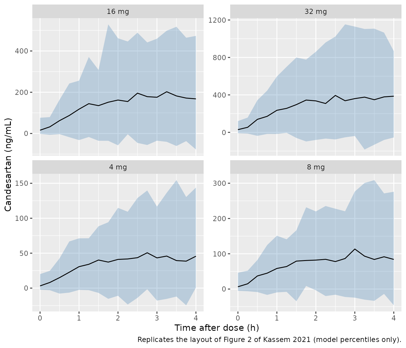
Figure 2: concentrations 0-4 h after a steady-state dose
Figure 2 of Kassem 2021 is a VPC between 0 and 4 h post-dose stratified by dose. The observed percentiles are not tabulated, so the panel below shows the model-predicted 2.5th, 50th and 97.5th percentiles (with residual error) for each dose at steady state, for visual comparison with the published figure.
vpc_subj <- subjects |> slice_head(n = 100)
doses <- c(4, 8, 16, 32)
ss_time <- 24 * 9 # 10 daily doses; the terminal half-life is about 5-10 h
obs_grid <- ss_time + seq(0, 4, by = 0.25)

ev_vpc <- bind_rows(lapply(seq_along(doses), function(i) {
  s <- vpc_subj |> mutate(id = id + (i - 1L) * 1000L, dose_mg = doses[i])
  bind_rows(
    tidyr::expand_grid(s, time = seq(0, ss_time, by = 24)) |>
      mutate(amt = dose_mg, evid = 1L, cmt = "depot"),
    tidyr::expand_grid(s, time = obs_grid) |>
      mutate(amt = NA_real_, evid = 0L, cmt = "central")
  )
})) |>
  arrange(id, time, desc(evid))

rxode2::rxSetSeed(20210103)
sim_vpc <- rxode2::rxSolve(
  mod,
  events = ev_vpc,
  omega = mod$omega,
  keep = c("dose_mg"),
  addDosing = FALSE
) |>
  as.data.frame() |>
  mutate(tad = time - ss_time)

sim_vpc |>
  group_by(dose_mg, tad) |>
  summarise(
    lo = quantile(sim, 0.025), med = median(sim), hi = quantile(sim, 0.975),
    .groups = "drop"
  ) |>
  ggplot(aes(tad, med)) +
  geom_ribbon(aes(ymin = lo, ymax = hi), fill = "steelblue", alpha = 0.3) +
  geom_line() +
  facet_wrap(~ paste(dose_mg, "mg"), scales = "free_y") +
  labs(
    x = "Time after dose (h)", y = "Candesartan (ng/mL)",
    caption = "Replicates the layout of Figure 2 of Kassem 2021 (model percentiles only)."
  )
PKNCA validation
The paper simulated each patient for 72 h after a dose and estimated the terminal half-life by log-linear regression, reporting 6.2 h (range 4-18 h). The same analysis is run here with PKNCA after a single 4 mg or 32 mg dose.
nca_grid <- c(0, 0.25, 0.5, 1, 1.5, 2, 3, 4, 5, 6, 8, 10, 12, 16, 24, 36, 48, 60, 72)
nca_subj <- subjects |> slice_head(n = 100)

ev_nca <- bind_rows(lapply(c(4, 32), function(d) {
  s <- nca_subj |>
    mutate(id = id + ifelse(d == 4, 0L, 1000L), treatment = paste(d, "mg"), dose_mg = d)
  bind_rows(
    s |> mutate(time = 0, amt = dose_mg, evid = 1L, cmt = "depot"),
    tidyr::expand_grid(s, time = nca_grid) |>
      mutate(amt = NA_real_, evid = 0L, cmt = "central")
  )
})) |>
  arrange(id, time, desc(evid))

sim_nca <- rxode2::rxSolve(
  mod,
  events = ev_nca,
  omega = mod$omega,
  keep = c("treatment"),
  addDosing = FALSE
) |>
  as.data.frame() |>
  dplyr::filter(!is.na(Cc)) |>
  select(id, time, Cc, treatment)

stopifnot(all(sim_nca$time[!duplicated(sim_nca$id)] == 0))

dose_nca <- ev_nca |>
  dplyr::filter(evid == 1) |>
  select(id, time, amt, treatment)

conc_obj <- PKNCA::PKNCAconc(sim_nca, Cc ~ time | treatment + id, concu = "ng/mL", timeu = "h")
dose_obj <- PKNCA::PKNCAdose(dose_nca, amt ~ time | treatment + id, doseu = "mg")
intervals <- data.frame(
  start = 0, end = Inf,
  cmax = TRUE, tmax = TRUE, aucinf.obs = TRUE, half.life = TRUE
)
nca_res <- PKNCA::pk.nca(PKNCA::PKNCAdata(conc_obj, dose_obj, intervals = intervals))

nca_tbl <- as.data.frame(nca_res$result) |>
  dplyr::filter(PPTESTCD %in% c("cmax", "tmax", "aucinf.obs", "half.life")) |>
  group_by(treatment, PPTESTCD) |>
  summarise(median = median(PPORRES, na.rm = TRUE), .groups = "drop") |>
  tidyr::pivot_wider(names_from = PPTESTCD, values_from = median)

nca_tbl |>
  dplyr::rename(
    "Treatment" = treatment,
    "Cmax (ng/mL)" = cmax,
    "Tmax (h)" = tmax,
    "AUC0-inf (ng.h/mL)" = aucinf.obs,
    "Terminal t1/2 (h)" = half.life
  ) |>
knitr::kable(digits = 2, caption = "Median simulated single-dose NCA (100 virtual patients per dose).")| Treatment | AUC0-inf (ng.h/mL) | Cmax (ng/mL) | Terminal t1/2 (h) | Tmax (h) |
|---|---|---|---|---|
| 32 mg | 4432.51 | 373.4 | 5.31 | 4 |
| 4 mg | 563.28 | 47.3 | 5.32 | 4 |
hl_sim <- as.data.frame(nca_res$result) |>
  dplyr::filter(PPTESTCD == "half.life") |>
  group_by(treatment) |>
  summarise(PPTESTCD = "half.life", PPORRES = mean(PPORRES, na.rm = TRUE), .groups = "drop")

cmp <- nlmixr2lib::ncaComparisonTable(
  simulated = hl_sim,
  reference = data.frame(treatment = c("4 mg", "32 mg"), half.life = 6.2),
  by = "treatment",
  units = c(half.life = "h"),
  tolerance_pct = 20
)
knitr::kable(
  cmp,
  digits = 2,
  caption = "Mean simulated terminal half-life vs the 6.2 h reported in Kassem 2021 Results. * differs by more than 20%."
)| NCA parameter | treatment | Reference | Simulated | % diff |
|---|---|---|---|---|
| t½ (h) | 4 mg | 6.2 | 5.32 | -14.2% |
| t½ (h) | 32 mg | 6.2 | 5.32 | -14.2% |
# The model is linear, so the half-life does not depend on dose; its centre
# must sit near the published 6.2 h and at or above ln(2)/ka = 5.3 h.
hl_all <- as.data.frame(nca_res$result) |>
  dplyr::filter(PPTESTCD == "half.life") |>
  dplyr::pull(PPORRES)
stopifnot(
  abs(mean(hl_all, na.rm = TRUE) / 6.2 - 1) < 0.2,
  median(hl_all, na.rm = TRUE) > 5.0
)
The simulated mean terminal half-life sits about 14% below the published 6.2 h. Because ka carries no IIV, the terminal phase of most patients is the absorption half-life (5.3 h); only patients whose CL/F falls below ka x V/F = 1.6 L/h show a longer, elimination-limited terminal phase. The paper’s 6.2 h mean and 18 h upper range came from empirical Bayes estimates of each observed patient and from its own choice of regression window, neither of which is reproducible from the published tables.
Assumptions and deviations
- Dose unit. Doses are milligrams of candesartan cilexetil, as administered and as reported in the paper; no molecular-weight conversion to candesartan is applied. The week-0 2-h concentrations of Table 4 support this reading (see above).
-
Residual error scale. Table 2 reports the residual
error as variances (
sigma2); the model uses their square roots (additive SD 2.345 ng/mL, proportional SD 0.6465). The additive term is in ng/mL, the assay unit. The mixed error model is NONMEM’sY = F + eps1 + F * eps2with independent epsilons, which is nlmixr2’sadd() + prop()default (combined2). - Interindividual variability was estimated on CL/F only (Table 2); Vd/F, ka and the lag time have none.
-
eGFR method. The eGFR estimating equation is not
stated; values are in mL/min/1.73 m^2 (Table 1) and map to the
CRCLcolumn. - Virtual cohort. Weight and eGFR are drawn independently from the Table 1 means and SDs; their correlation in the real cohort is not reported. Diabetes is drawn independently of weight, although the paper notes that patients with diabetes were usually overweight.
-
Covariates screened but not retained (age,
NT-proBNP, furosemide, sex) are documented in the model’s
covariatesDataExcludedlist with their Supplementary Table S1 objective-function changes. - Scope. The paper’s separate men-only and women-only clearance analyses (structural model, no estimates beyond CL/F 7.96 vs 5.9 L/h) and its pharmacodynamic comparisons (Supplementary Tables S3-S4, statistical models of potassium, blood pressure and eGFR change) are not population PK/PD models and are not encoded.