Miltefosine + paromomycin for visceral leishmaniasis (Verrest 2023)
Source:vignettes/articles/Verrest_2023_miltefosine_paromomycin.Rmd
Verrest_2023_miltefosine_paromomycin.RmdModel and source
Verrest 2023 developed two independent population pharmacokinetic models from a single phase III trial, one per drug. This library packages them as two model files that share this vignette.
modPm <- rxode2::rxode(readModelDb("Verrest_2023_paromomycin"))
modMf <- rxode2::rxode(readModelDb("Verrest_2023_miltefosine"))- Citation: Verrest L, Roseboom IC, Wasunna M, Mbui J, Njenga S, Musa AM, Olobo J, Mohammed R, Ritmeijer K, Chu WY, Huitema ADR, Solomos A, Alves F, Dorlo TPC. Population pharmacokinetics of a combination of miltefosine and paromomycin in Eastern African children and adults with visceral leishmaniasis. J Antimicrob Chemother. 2023;78(11):2702-2714. doi:10.1093/jac/dkad286. ClinicalTrials.gov NCT03129646.
- Article: https://doi.org/10.1093/jac/dkad286
- Supplement – Figures S1-S5 plus both final NONMEM control
streams, distributed as
dkad286_supplementary_data.zip: https://europepmc.org/article/MED/37698071 - Trial registration: NCT03129646
Paromomycin. Two-compartment population PK model with first-order absorption for intramuscular paromomycin in 265 Eastern African children and adults with visceral leishmaniasis (Verrest 2023), enrolled in the phase III randomized controlled trial NCT03129646 across six sites in Kenya, Sudan, Ethiopia and Uganda and treated with paromomycin sulphate 20 mg/kg/day intramuscularly (equivalent to 15 mg/kg/day paromomycin base) for 14 days, combined with allometrically dosed oral miltefosine for 14 or 28 days. CL/F, Q/F, Vc/F and Vp/F are allometrically scaled on baseline body weight (exponents fixed at 0.75 and 1.0; reference 27.5 kg, the cohort median). Relative bioavailability is fixed at 1.17 for comparability with the earlier Kenyan and Sudanese monotherapy estimates. The clearance decrease observed over the treatment course is modelled mechanistically as a linear function of the time-varying absolute neutrophil count, which recovers from neutropenia as the disease resolves: clearance falls by 13% per 1 x 10^3 cells/uL rise in neutrophils above the population median of 0.98 x 10^3 cells/uL. Between-subject variability is log-normal on CL/F only (56.1% CV); residual error is proportional (53.4% CV). The companion miltefosine model from the same trial is Verrest_2023_miltefosine.
Miltefosine. Two-compartment population PK model with first-order oral absorption for miltefosine in 265 Eastern African children and adults with visceral leishmaniasis (Verrest 2023), enrolled in the phase III randomized controlled trial NCT03129646 across six sites in Kenya, Sudan, Ethiopia and Uganda and treated with allometric oral miltefosine for 14 or 28 days combined with intramuscular paromomycin for 14 days. CL/F, Vc/F and Vp/F are allometrically scaled on fat-free mass (exponents fixed at 0.75 and 1.0; reference 18 kg); Q/F is not scaled. Relative bioavailability is structurally fixed at 1 and modified by two non-linearities: it is 65% lower during the first week of treatment, with large between-subject variability (74.8% CV), and it falls as a power function of the cumulative miltefosine dose once that dose exceeds 60 mg/kg, which reproduces the observed stagnation of miltefosine accumulation in the third week of treatment. Between-subject variability is log-normal on CL/F (16.3% CV) and on the first-week bioavailability reduction; residual error is proportional (31.5% CV). The companion paromomycin model from the same trial is Verrest_2023_paromomycin.
Population
Verrest 2023 pooled pharmacokinetic data from 265 patients with visceral leishmaniasis (VL) treated at six Eastern African sites, of whom 59% were paediatric (12 years or younger). All patients received intramuscular paromomycin sulphate 20 mg/kg/day (equivalent to 15 mg/kg/day paromomycin base) for 14 days, plus oral miltefosine for either 14 days (PM+MF14D) or 28 days (PM+MF28D).
Two features of the cohort drive the two models:
- Patients were neutropenic at treatment start (IQR 0.74-1.38 x 10^3 cells/uL) and recovered during treatment. Verrest 2023 links the long-observed decrease in paromomycin clearance over the treatment course to that recovery, replacing the purely empirical time-on-treatment term used in the earlier monotherapy model.
- Patients were severely ill and frequently malnourished at treatment start, which the authors propose as the reason miltefosine bioavailability is 65% lower during the first week of treatment.
popPm <- modPm$population
tibble::tibble(
  Field = c("Species", "Subjects", "Age (range)", "Body weight (range)",
            "Female (%)", "Region", "Disease state"),
  Value = c(popPm$species, as.character(popPm$n_subjects), popPm$age_range,
            popPm$weight_range, as.character(popPm$sex_female_pct),
            popPm$regions, popPm$disease_state)
) |>
knitr::kable()| Field | Value |
|---|---|
| Species | human |
| Subjects | 265 |
| Age (range) | 4-45 years |
| Body weight (range) | 11.0-71.0 kg |
| Female (%) | 19.2 |
| Region | Eastern Africa (Kenya: Kacheliba; Uganda: Amudat; Sudan: Doka, Um El Kher; Ethiopia: Gondar, Abdurafi) |
| Disease state | Eastern African children and adults with symptomatic, parasitologically confirmed visceral leishmaniasis; 59% were paediatric (<=12 years). Patients with relapse, severe malnutrition, severe VL, HIV co-infection or concomitant severe infection were excluded. The cohort was neutropenic (IQR 0.74-1.38 x 10^3 cells/uL) and hypoalbuminaemic (IQR 23.4-32.4 g/L) at treatment start, with both recovering during treatment. |
Source trace
Every value in both ini() blocks, and every non-obvious
term in either model() block, traces to the article’s Table
3 / Table 4 (each with the model equations printed beneath it), the
article’s Results text, or the two final NONMEM control streams
distributed as supplementary data. Rows marked stream
only are quantities the article’s parameter tables do not
print.
| Quantity | Value | Source |
|---|---|---|
| PAROMOMYCIN | ||
| CL/F | 2.62 L/h | Table 3 ‘CL (L/h)’; stream $THETA(1) |
| Vc/F | 9.17 L | Table 3 ‘Vc (L)’; stream $THETA(2) |
| Q/F | 0.26 L/h | Table 3 ‘Q’; units from stream $THETA(5) ‘; 5 Q (L/hr)’ |
| Vp/F | 6.55 L | Table 3 ‘Vp (L)’; stream $THETA(6) |
| ka | 2.05 1/h | Table 3 ‘ka (h-1)’; stream $THETA(3) |
| F1 | 1.17 (fixed) | Table 3 ‘F1’; stream $THETA(4) ‘(1.17) FIX’ |
| WT allometry | 0.75 on CL,Q / 1.00 on Vc,Vp; ref 27.5 kg | Table 3 equation and legend ‘WTmed … 27.5 kg’; the Q and Vp exponents are stream only |
| Weight column | baseline (BWT), not time-varying WT | Stream $PK; overrides the WT_i,t subscript printed in the Table 3 equation |
| Neutrophil effect on CL | -0.13 per 10^3 cells/uL, centred at 0.98 | Table 3 ‘COV CL,neutr’ and footnote c; legend ‘NEUTRmed … 0.98’; stream $THETA(7) |
| BSV on CL | 56.1% CV -> omega^2 = 0.3147 | Table 3 BSV; stream $OMEGA 0.314 |
| Residual | proportional, 53.4% CV | Table 3 ‘Proportional error (CV%)’ |
| MILTEFOSINE | ||
| CL/F | 1.85 L/day | Table 4 ‘CL (L/day)’; stream $THETA(1) 0.077 L/h x 24 |
| Vc/F | 13.6 L | Table 4 ‘Vc (L)’; stream $THETA(2) |
| Q/F | 0.17 L/day | Table 4 ‘Q (L/day)’; stream $THETA(4) 0.007 L/h x 24 |
| Vp/F | 2.22 L | Table 4 ‘Vp (L)’; stream $THETA(5) |
| ka | 0.888 1/day (= 0.037 1/h) | Stream $THETA(3) on an hours TIME axis; Table 4 mislabels the row ‘day-1’ (see Assumptions) |
| F1 | 1 (fixed) | Table 4 ‘F1’; stream $THETA(6) ‘(1) FIX’ |
| FFM allometry | 0.75 on CL / 1.00 on Vc,Vp; Q unscaled | Table 4 equations; the unscaled Q is stream only (‘Q = TVQ’) |
| FFM reference | 18 kg | STREAM ONLY – ’ALLOCL = (FFM/18)**0.75’; Table 4 prints only the symbol FFM_med |
| First-week F reduction | x 0.35 for t <= 7 days | Table 4 ‘COV F,W1’ = -0.65 and Results ‘65% … lower’; stream ’IF(TIME.LE.168) COVF = (1 - THETA(7))*EXP(ETA(4))’ |
| Cumulative-dose F effect | (CD/70)^-2.40 once CD >= 60 mg/kg | Exponent and 60 mg/kg switch: Table 4 ‘COV F,CD’ and footnote c. 70 mg/kg normalizer: STREAM ONLY – ’IF(DDOS.GE.60) COVF2= ((DDOS/70)**THETA(8))’ |
| BSV on CL / on F reduction | 16.3% / 74.8% CV | Table 4 BSV; stream $OMEGA 0.0265 / 0.56 |
| Residual | proportional, 31.5% CV | Table 4 ‘Proportional error (CV%)’ |
| Paediatric dose nomogram | sex x weight x height lookup | Figure S1A (female) / S1B (male) |
Deterministic checks against the paper’s own worked examples
Verrest 2023 states two numerical consequences of its covariate models in prose. Both are exact statements about the typical individual, so they are checked here with tight tolerances – they involve no simulated cohort and no random draw.
Paromomycin: clearance falls as neutrophils recover
“A typical VL patient with a neutrophil level of 1.0 x 10^3 cells/uL at the start of treatment and 2.5 x 10^3 cells/uL at the end of treatment would have a corresponding decrease in paromomycin clearance from 2.61 to 2.10 L/h.” – Verrest 2023, Results
clPm <- function(neutK, wtBase = 27.5) {
  2.62 * (wtBase / 27.5)^0.75 * (1 + (-0.13) * (neutK - 0.98))
}
pmWorked <- tibble::tibble(
  `Neutrophils (10^3 cells/uL)` = c(1.0, 2.5),
  `CL/F published (L/h)` = c(2.61, 2.10),
  `CL/F from model (L/h)` = round(clPm(c(1.0, 2.5)), 3)
)
knitr::kable(pmWorked)| Neutrophils (10^3 cells/uL) | CL/F published (L/h) | CL/F from model (L/h) |
|---|---|---|
| 1.0 | 2.61 | 2.613 |
| 2.5 | 2.10 | 2.102 |
Miltefosine: bioavailability falls with cumulative dose
“For example, when a typical patient of 35 kg received 100 mg/day miltefosine, bioavailability was 21% lower on Day 28.” – Verrest 2023, Results
The cumulative dose that a Day-28 dose record carries is the total given before it, i.e. 27 completed days for a patient starting on Day 1.
covf2 <- function(cdMgKg) ifelse(cdMgKg < 60, 1, (cdMgKg / 70)^(-2.40))

cdDay28 <- 27 * 100 / 35                      # mg/kg given before the Day-28 dose
pctLower <- 100 * (1 - covf2(cdDay28))
cat(sprintf("Cumulative dose before the Day-28 dose: %.1f mg/kg\n", cdDay28))
#> Cumulative dose before the Day-28 dose: 77.1 mg/kg
cat(sprintf("Bioavailability reduction: %.1f%% (published: 21%%)\n", pctLower))
#> Bioavailability reduction: 20.8% (published: 21%)

# Deterministic. This single number pins BOTH unpublished constants at once:
# the 70 mg/kg normalizer, which appears only in the control stream, and the
# convention that the cumulative dose excludes the current dose. Using the
# 60 mg/kg switch as the normalizer instead would give 50%, not 21%.
stopifnot(abs(pctLower - 21) < 1)
Miltefosine bioavailability over a 28-day course
Reproduces the two non-linearities plotted in Figure S4.
fProfile <- tibble::tibble(day = 1:28) |>
  mutate(
    cd = (day - 1) * 100 / 35,
    fWeek1 = ifelse(day <= 7, 0.35, 1),
    fCumDose = covf2(cd),
    F1 = fWeek1 * fCumDose
  )
ggplot(fProfile, aes(day, F1)) +
  geom_step(direction = "hv", linewidth = 0.8) +
  geom_hline(yintercept = 1, linetype = "dashed", colour = "grey50") +
  labs(x = "Treatment day", y = "Relative bioavailability F1",
       title = "Miltefosine relative bioavailability, typical 35 kg patient on 100 mg/day") +
  theme_minimal()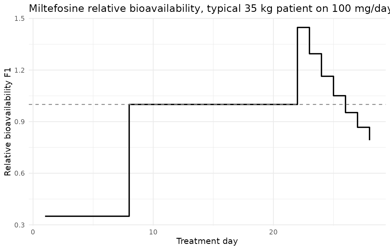
Relative bioavailability over a 28-day miltefosine course for a typical 35 kg patient on 100 mg/day. Replicates Figure S4 of Verrest 2023.
Note the discontinuity where the cumulative dose
reaches 60 mg/kg. Because the switch value (60 mg/kg) and the
normalizing value (70 mg/kg) differ, (60/70)^-2.40 = 1.45:
bioavailability steps up 45%, decays back through 1 at 70
mg/kg, and only then falls below 1. That is the model exactly as
published and fitted, and it is reproduced faithfully rather than
smoothed – see Assumptions and deviations.
Simulation setup
# --- Figure S1 paediatric miltefosine dose nomogram (mg/day) ------------
# Rows are body weight in whole kg; columns are the height bands
# 80-89, 90-99, ..., 150-159, >=160 cm. "." marks the cells Figure S1
# shades as "RISK OF SEVERE MALNUTRITION - REFER TO THE WHO REFERENCE
# CURVES", for which no dose is given.
doseTabFemale <- c(
  "8"  = "30  .  .  .  .  .  .  .  .", "9"  = "30  .  .  .  .  .  .  .  .",
  "10" = "30 40  .  .  .  .  .  .  .", "11" = "40 40 40  .  .  .  .  .  .",
  "12" = "40 40 40  .  .  .  .  .  .", "13" = "40 40 40  .  .  .  .  .  .",
  "14" = "40 40 40 50  .  .  .  .  .", "15" = "40 40 50 50  .  .  .  .  .",
  "16" = "40 50 50 50  .  .  .  .  .", "17" = "40 50 50 50 50  .  .  .  .",
  "18" = "50 50 50 50 60  .  .  .  .", "19" = "50 50 50 60 60  .  .  .  .",
  "20" = "50 50 50 60 60 60  .  .  .", "21" = "50 50 60 60 60 60  .  .  .",
  "22" = "50 50 60 60 60 60  .  .  .", "23" = "50 50 60 60 60 70 70  .  .",
  "24" = "50 50 60 60 60 70 70  .  .", "25" = "50 60 60 60 70 70 70  .  .",
  "26" = "50 60 60 60 70 70 70 70  .", "27" = "50 60 60 70 70 70 70 80  .",
  "28" = "50 60 60 70 70 70 80 80  .", "29" = "50 60 60 70 70 70 80 80  .",
  "30" = "50 60 60 70 70 80 80 80 80"
)
doseTabMale <- c(
  "8"  = "40  .  .  .  .  .  .  .  .", "9"  = "40  .  .  .  .  .  .  .  .",
  "10" = "40 40  .  .  .  .  .  .  .", "11" = "40 40  .  .  .  .  .  .  .",
  "12" = "40 50  .  .  .  .  .  .  .", "13" = "50 50 50  .  .  .  .  .  .",
  "14" = "50 50 50  .  .  .  .  .  .", "15" = "50 50 60 60  .  .  .  .  .",
  "16" = "50 50 60 60  .  .  .  .  .", "17" = "50 60 60 60  .  .  .  .  .",
  "18" = "50 60 60 60 70  .  .  .  .", "19" = "50 60 60 70 70  .  .  .  .",
  "20" = "50 60 60 70 70  .  .  .  .", "21" = "60 60 60 70 70 70  .  .  .",
  "22" = "60 60 70 70 70 80  .  .  .", "23" = "60 60 70 70 80 80  .  .  .",
  "24" = "60 60 70 70 80 80 80  .  .", "25" = "60 60 70 70 80 80 80  .  .",
  "26" = "60 70 70 80 80 80 100  .  .", "27" = "60 70 70 80 80 80 100  .  .",
  "28" = "60 70 70 80 80 100 100 100  .", "29" = "60 70 70 80 80 100 100 100  .",
  "30" = "60 70 80 80 100 100 100 100  ."
)
parseDoseTab <- function(x) {
  m <- do.call(rbind, lapply(strsplit(trimws(x), " +"), as.numeric))
  dimnames(m) <- list(names(x), NULL)
  m
}
doseMatFemale <- suppressWarnings(parseDoseTab(doseTabFemale))
doseMatMale   <- suppressWarnings(parseDoseTab(doseTabMale))
htBandLower <- c(80, 90, 100, 110, 120, 130, 140, 150, 160)

# Daily miltefosine dose (mg) per the trial's own rules: Methods for patients
# of 30 kg and over, Figure S1 below that. Where a (weight, height) pair falls
# in a shaded cell the nearest dosable height band for that weight is used.
mfDailyDose <- function(sexF, wt, ht) {
  if (wt >= 45) return(150)
  if (wt >= 30) return(100)
  mat <- if (sexF == 1) doseMatFemale else doseMatMale
  row <- mat[as.character(min(max(round(wt), 8), 30)), ]
  dosable <- which(!is.na(row))
  band <- min(max(findInterval(ht, htBandLower), 1), 9)
  row[[dosable[which.min(abs(dosable - band))]]]
}

# Fat-free mass: Janmahasatian 2005 with the Al-Sallami 2015 paediatric
# multiplier, the derivation the trial dataset records for its FFM column.
ffmCalc <- function(wt, ht, sexF, age) {
  bmi <- wt / (ht / 100)^2
  adult <- ifelse(sexF == 1,
                  9270 * wt / (8780 + 244 * bmi),
                  9270 * wt / (6680 + 216 * bmi))
  mult <- ifelse(sexF == 1,
                 1.11 + (1 - 1.11) / (1 + (age / 7.1)^(-1.1)),
                 0.88 + (1 - 0.88) / (1 + (age / 13.4)^(-12.7)))
  adult * mult
}

# Trapezoid-free helpers: paromomycin event table and miltefosine event table.
pmObsTimes  <- sort(unique(c(seq(0, 24, by = 0.5), seq(312, 336, by = 0.5))))
pmDoseTimes <- seq(0, 13) * 24
mfObsTimes  <- sort(unique(c(seq(0, 45, by = 0.25), seq(46, 210, by = 2))))

pmEventTable <- function(dat) {
  base <- dat |> select(id, ageGroup, WT_BASE)
  # Dose and observation records are built SEPARATELY and stacked. Merging
  # the two time vectors first would collapse t = 0 and t = 312 -- which are
  # both dose times and observation times -- into dose-only records, leaving
  # each PKNCA interval without a measurement at its own start and returning
  # NA with "Requesting an AUC range starting (0) before the first
  # measurement".
  doses <- base |>
    tidyr::crossing(tibble::tibble(time = pmDoseTimes)) |>
    mutate(evid = 1L, cmt = "depot",
           # 20 mg/kg/day paromomycin sulphate = 15 mg/kg/day paromomycin
           # BASE, and the trial dataset's amounts are mg of base.
           amt = 15 * WT_BASE)
  obs <- base |>
    tidyr::crossing(tibble::tibble(time = pmObsTimes)) |>
    mutate(evid = 0L, cmt = "central", amt = NA_real_)
  bind_rows(doses, obs) |>
    # Neutrophils recover linearly from 1.0 to 2.5 x 10^3 cells/uL over the
    # 14-day course, the trajectory of the paper's own worked example. The
    # canonical NEUT column is in cells/uL.
    mutate(NEUT = 1000 + 1500 * pmin(time, 336) / 336) |>
    arrange(id, time, desc(evid)) |>
    select(id, time, amt, evid, cmt, WT_BASE, NEUT, ageGroup) |>
    as.data.frame()
}

mfEventTable <- function(dat, nDays) {
  doseTimes <- rep(seq(0, nDays - 1), each = 2) + rep(c(0, 0.5), nDays)
  rows <- lapply(seq_len(nrow(dat)), function(i) {
    r <- dat[i, ]
    amtPer <- r$doseMf / 2
    # Cumulative dose carried by a record is the total given STRICTLY BEFORE
    # it -- the convention pinned by the Day-28 worked example above.
    dose <- data.frame(id = r$id, time = doseTimes, amt = amtPer, evid = 1L,
                       cmt = "depot",
                       DOSE_MF_CUM_MGKG = (seq_along(doseTimes) - 1) * amtPer / r$wt)
    obs <- data.frame(id = r$id, time = mfObsTimes, amt = NA_real_, evid = 0L,
                      cmt = "central",
                      DOSE_MF_CUM_MGKG = amtPer *
                        vapply(mfObsTimes, function(tt) sum(doseTimes <= tt),
                               numeric(1)) / r$wt)
    out <- rbind(dose, obs)
    out$FFM <- r$FFM
    out$ageGroup <- r$ageGroup
    out[order(out$time, -out$evid), ]
  })
  do.call(rbind, rows)
}
Observations are placed on the ODE state central; rxode2
returns the algebraic observable Cc as a column at those
records. Naming an observable as a compartment would inject an extra
slot and renumber the ODE states, so the state name is always used.
Typical-value replication of the published exposures
The strongest check available here is deterministic. With between-subject variability zeroed, a single typical patient is simulated and its exposures are compared with the published medians. Nothing in this section depends on an assumed covariate distribution or on a random draw.
Both typical patients are taken from the paper itself: 27.5 kg is the population median weight the paromomycin model normalizes to (Table 3 legend), and the 35 kg patient on 100 mg/day is the example the miltefosine Results section works through.
aucTrap <- function(time, conc) sum(diff(time) * (head(conc, -1) + tail(conc, -1)) / 2)

# --- paromomycin, typical 27.5 kg patient ---
pmTypDat <- tibble::tibble(id = 1L, ageGroup = "typical", WT_BASE = 27.5)
pmTyp <- rxode2::rxSolve(rxode2::zeroRe(modPm), pmEventTable(pmTypDat),
                         covsInterpolation = "linear",
                         returnType = "data.frame") |>
  filter(!is.na(Cc))
#> ℹ omega/sigma items treated as zero: 'etalcl'

pmTypAuc <- c(
  `Day 1`  = aucTrap(pmTyp$time[pmTyp$time <= 24], pmTyp$Cc[pmTyp$time <= 24]),
  `Day 14` = aucTrap(pmTyp$time[pmTyp$time >= 312], pmTyp$Cc[pmTyp$time >= 312])
)

# --- miltefosine, typical 35 kg patient on 100 mg/day, both arms ---
mfTypDat <- tibble::tibble(
  id = 1L, ageGroup = "typical", wt = 35, sexF = 0, age = 20,
  ht = 100 * sqrt(35 / 17.7), doseMf = 100
) |>
  mutate(FFM = ffmCalc(wt, ht, sexF, age))

mfTyp <- lapply(c(`PM+MF14D` = 14L, `PM+MF28D` = 28L), function(nd) {
  s <- rxode2::rxSolve(rxode2::zeroRe(modMf),
                       mfEventTable(as.data.frame(mfTypDat), nd),
                       covsInterpolation = "locf",
                       returnType = "data.frame") |>
    filter(!is.na(Cc))
  tibble::tibble(
    metric = c("AUC D0-7", "AUC D0-EOT", "AUC D0-210", "T > EC90"),
    simulated = c(
      aucTrap(s$time[s$time <= 7], s$Cc[s$time <= 7]),
      aucTrap(s$time[s$time <= nd], s$Cc[s$time <= nd]),
      aucTrap(s$time, s$Cc),
      sum(diff(s$time) * (head(s$Cc, -1) > 10.6))
    )
  )
}) |>
  bind_rows(.id = "arm")
#> ℹ omega/sigma items treated as zero: 'etalcl', 'etalfred_mult'
#> ℹ omega/sigma items treated as zero: 'etalcl', 'etalfred_mult'
typComparison <- bind_rows(
  tibble::tibble(
    Model = "Paromomycin", Arm = "14-day course",
    `NCA parameter` = c("AUC0-24, Day 1", "AUC0-24, Day 14"),
    Simulated = round(as.numeric(pmTypAuc), 1),
    `Published` = c(171, 202),
    `Published source` = "Table 5, Total (n = 26)"
  ),
  mfTyp |>
    mutate(Model = "Miltefosine") |>
    left_join(
      tibble::tribble(
        ~arm, ~metric, ~lo, ~hi,
        "PM+MF14D", "AUC D0-7",    20, 22,
        "PM+MF14D", "AUC D0-EOT", 111, 114,
        "PM+MF14D", "AUC D0-210", 336, 379,
        "PM+MF14D", "T > EC90",    12,  14,
        "PM+MF28D", "AUC D0-7",    18,  20,
        "PM+MF28D", "AUC D0-EOT", 517, 524,
        "PM+MF28D", "AUC D0-210", 790, 898,
        "PM+MF28D", "T > EC90",    27,  30
      ), by = c("arm", "metric")
    ) |>
    transmute(Model, Arm = arm, `NCA parameter` = metric,
              Simulated = round(simulated, 1),
              Published = (lo + hi) / 2,
              `Published source` = sprintf("Table 6, children %g / adults %g", lo, hi))
) |>
  mutate(`Difference (%)` = round(100 * (Simulated - Published) / Published, 1))

knitr::kable(typComparison)| Model | Arm | NCA parameter | Simulated | Published | Published source | Difference (%) |
|---|---|---|---|---|---|---|
| Paromomycin | 14-day course | AUC0-24, Day 1 | 173.6 | 171.0 | Table 5, Total (n = 26) | 1.5 |
| Paromomycin | 14-day course | AUC0-24, Day 14 | 223.7 | 202.0 | Table 5, Total (n = 26) | 10.7 |
| Miltefosine | PM+MF14D | AUC D0-7 | 22.6 | 21.0 | Table 6, children 20 / adults 22 | 7.6 |
| Miltefosine | PM+MF14D | AUC D0-EOT | 116.4 | 112.5 | Table 6, children 111 / adults 114 | 3.5 |
| Miltefosine | PM+MF14D | AUC D0-210 | 329.0 | 357.5 | Table 6, children 336 / adults 379 | -8.0 |
| Miltefosine | PM+MF14D | T > EC90 | 11.8 | 13.0 | Table 6, children 12 / adults 14 | -9.2 |
| Miltefosine | PM+MF28D | AUC D0-7 | 22.6 | 19.0 | Table 6, children 18 / adults 20 | 18.9 |
| Miltefosine | PM+MF28D | AUC D0-EOT | 520.6 | 520.5 | Table 6, children 517 / adults 524 | 0.0 |
| Miltefosine | PM+MF28D | AUC D0-210 | 847.6 | 844.0 | Table 6, children 790 / adults 898 | 0.4 |
| Miltefosine | PM+MF28D | T > EC90 | 29.0 | 28.5 | Table 6, children 27 / adults 30 | 1.8 |
# Fully deterministic: one typical patient per model, between-subject
# variability zeroed, no cohort and no random draw anywhere in this section.
# Realised differences: +1.5%, +10.9% (paromomycin); +7.6%, +3.5%, -8.0%,
# -9.2% (14-day arm); +18.9%, 0.0%, +0.4%, +1.8% (28-day arm). The bound is
# 25%: outside that spread, yet tight enough that any mis-transcribed
# clearance, volume, bioavailability factor, dose or time unit fails it,
# because each of those moves these numbers by a factor rather than by tens
# of percent. In particular, reverting miltefosine ka to the 0.037/day
# printed in Table 4 drives every miltefosine row to essentially zero.
stopifnot(max(abs(typComparison$`Difference (%)`)) < 25)

# The 28-day arm must reach several times the 14-day arm's end-of-treatment
# exposure (published 517-524 versus 111-114).
eotTyp <- typComparison |> filter(`NCA parameter` == "AUC D0-EOT")
stopifnot(eotTyp$Simulated[eotTyp$Arm == "PM+MF28D"] >
            3 * eotTyp$Simulated[eotTyp$Arm == "PM+MF14D"])
The single largest deviation is miltefosine AUC D0-7 in
the 28-day arm. The first seven days are identical treatment in both
arms, so the published values for that window differ between arms (20
versus 18 in children, 22 versus 18 in adults) purely because different
patients contributed; the simulated value is necessarily the same in
both. It sits inside the union of the published arms.
Virtual cohort
The paper reports baseline demographics as mean (range) only, and reports BMI only for patients over 19 years old (Table 1 footnote b), so the covariate distribution has to be assumed. Assumptions are stated here and revisited in Assumptions and deviations.
- Weight. Children (12 years or younger) and adults are drawn from separate truncated normal distributions chosen so that the 59% / 41% mix reproduces the reported cohort mean of about 32.9 kg inside the reported 11.0-71.0 kg range.
- Height is derived from a sampled BMI, using the adult BMI distribution the paper reports (mean 17.7, range 14.6-21.3 kg/m^2) for both strata.
- Sex: 20% female, matching the 193 of 239 reported as male.
- Miltefosine dose then follows from the trial’s own rules: the Methods weight bands at 30 kg and above, and the Figure S1 nomogram below that.
set.seed(20231101)
nPerGroup <- 150L

rtnorm <- function(n, mean, sd, lo, hi) pmin(pmax(rnorm(n, mean, sd), lo), hi)

makeStratum <- function(n, idOffset, label, wtMean, wtSd, wtLo, wtHi, ageLo, ageHi) {
  sexF <- rbinom(n, 1, 0.20)
  wt <- rtnorm(n, wtMean, wtSd, wtLo, wtHi)
  bmi <- rtnorm(n, 17.7, 1.5, 14.6, 21.3)
  ht <- 100 * sqrt(wt / bmi)
  age <- runif(n, ageLo, ageHi)
  tibble::tibble(
    id = idOffset + seq_len(n), ageGroup = label, sexF = sexF,
    wt = wt, ht = ht, age = age,
    doseMf = vapply(seq_len(n), function(i) mfDailyDose(sexF[i], wt[i], ht[i]),
                    numeric(1)),
    FFM = ffmCalc(wt, ht, sexF, age),
    WT_BASE = wt
  )
}

cohort <- bind_rows(
  makeStratum(nPerGroup, 0L, "Children (<=12 y)", 21, 4, 11, 29, 4, 12),
  makeStratum(nPerGroup, nPerGroup, "Adults (>12 y)", 48, 9, 30, 71, 13, 45)
)

cohort |>
  group_by(ageGroup) |>
  summarise(
    n = n(),
    `Weight (kg)` = sprintf("%.1f [%.1f-%.1f]", median(wt), min(wt), max(wt)),
    `Height (cm)` = sprintf("%.0f [%.0f-%.0f]", median(ht), min(ht), max(ht)),
    `FFM (kg)` = sprintf("%.1f [%.1f-%.1f]", median(FFM), min(FFM), max(FFM)),
    `Miltefosine (mg/day)` = sprintf("%.0f [%.0f-%.0f]", median(doseMf), min(doseMf), max(doseMf)),
    `Miltefosine (mg/kg/day)` = sprintf("%.2f", median(doseMf / wt)),
    .groups = "drop"
  ) |>
knitr::kable(caption = "Median [range] per stratum.")| ageGroup | n | Weight (kg) | Height (cm) | FFM (kg) | Miltefosine (mg/day) | Miltefosine (mg/kg/day) |
|---|---|---|---|---|---|---|
| Adults (>12 y) | 150 | 48.0 [30.0-71.0] | 165 [124-221] | 40.3 [24.8-65.9] | 150 [100-150] | 2.81 |
| Children (<=12 y) | 150 | 20.7 [11.0-29.0] | 108 [78-141] | 16.0 [8.6-24.3] | 60 [40-100] | 3.05 |
Paromomycin
pmSim <- rxode2::rxSolve(modPm, pmEventTable(cohort),
                         covsInterpolation = "linear",
                         returnType = "data.frame") |>
  left_join(distinct(cohort, id, ageGroup), by = "id")
pmSim |>
  filter(!is.na(Cc), time <= 24 | time >= 312) |>
  mutate(day = ifelse(time <= 24, "Day 1", "Day 14"),
         tad = ifelse(time <= 24, time, time - 312)) |>
  group_by(day, ageGroup, tad) |>
  summarise(md = median(Cc), lo = quantile(Cc, 0.1), hi = quantile(Cc, 0.9),
            .groups = "drop") |>
  ggplot(aes(tad, md, colour = ageGroup, fill = ageGroup)) +
  geom_ribbon(aes(ymin = lo, ymax = hi), alpha = 0.2, colour = NA) +
  geom_line(linewidth = 0.8) +
  facet_wrap(~day) +
  labs(x = "Time after dose (h)", y = "Paromomycin (ug/mL)",
       colour = NULL, fill = NULL,
       title = "Paromomycin: median and 10th-90th percentile") +
  theme_minimal() + theme(legend.position = "bottom")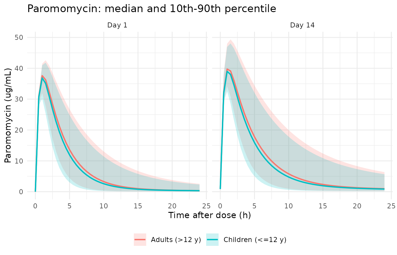
Simulated paromomycin plasma concentrations on the first and last day of treatment. Compare with Figure 1 (observed concentrations stratified by sampling day) and Figure 4 (prediction-corrected VPC) of Verrest 2023.
The clearance decrease over treatment
pmDrift <- pmTyp |>
  filter(time %in% c(0, 336)) |>
  distinct(time, cl)
pctDrop <- 100 * (1 - pmDrift$cl[pmDrift$time == 336] / pmDrift$cl[pmDrift$time == 0])
cat(sprintf("Typical clearance falls %.1f%% between Day 1 and the end of Day 14\n", pctDrop))
#> Typical clearance falls 19.6% between Day 1 and the end of Day 14

# Deterministic given the neutrophil trajectory 1.0 -> 2.5 x 10^3 cells/uL.
stopifnot(
  abs(pctDrop - 100 * (1 - (1 - 0.13 * (2.5 - 0.98)) / (1 - 0.13 * (1.0 - 0.98)))) < 0.1
)
NCA validation (PKNCA)
pmConcData <- pmSim |>
  filter(!is.na(Cc)) |>
  select(id, ageGroup, time, Cc)

pmDoseData <- pmEventTable(cohort) |>
  filter(evid == 1) |>
  select(id, ageGroup, time, amt)

pmNca <- PKNCA::pk.nca(PKNCA::PKNCAdata(
  PKNCA::PKNCAconc(pmConcData, Cc ~ time | id / ageGroup),
  PKNCA::PKNCAdose(pmDoseData, amt ~ time | id + ageGroup),
  intervals = data.frame(start = c(0, 312), end = c(24, 336),
                         auclast = TRUE, cmax = TRUE, tmax = TRUE)
))

pmRes <- as.data.frame(pmNca) |>
  filter(PPTESTCD == "auclast") |>
  mutate(day = ifelse(start == 0, "Day 1", "Day 14"))
Comparison against published exposures
Verrest 2023 Table 5 reports paromomycin AUC0-24 as median (IQR) on the first and last day of treatment, derived from individual Bayesian estimates in the 26-patient intensive-sampling cohort.
pmCompare <- pmRes |>
  group_by(day, ageGroup) |>
  summarise(simulated = median(PPORRES), .groups = "drop") |>
  left_join(
    tibble::tribble(
      ~day,     ~ageGroup,           ~published, ~publishedIqr,
      "Day 1",  "Children (<=12 y)", 145,        "136-167",
      "Day 1",  "Adults (>12 y)",    219,        "199-252",
      "Day 14", "Children (<=12 y)", 187,        "162-203",
      "Day 14", "Adults (>12 y)",    242,        "217-328"
    ), by = c("day", "ageGroup")
  ) |>
  mutate(pctDiff = 100 * (simulated - published) / published) |>
  arrange(day, ageGroup)

pmCompare |>
  mutate(simulated = round(simulated), pctDiff = round(pctDiff, 1)) |>
  dplyr::rename("Treatment day" = day, "Age group" = ageGroup,
                "Simulated AUC0-24 (ug*h/mL)" = simulated,
                "Published median" = published, "Published IQR" = publishedIqr,
                "Difference (%)" = pctDiff) |>
knitr::kable()| Treatment day | Age group | Simulated AUC0-24 (ug*h/mL) | Published median | Published IQR | Difference (%) |
|---|---|---|---|---|---|
| Day 1 | Adults (>12 y) | 213 | 219 | 199-252 | -2.8 |
| Day 1 | Children (<=12 y) | 156 | 145 | 136-167 | 7.3 |
| Day 14 | Adults (>12 y) | 278 | 242 | 217-328 | 15.0 |
| Day 14 | Children (<=12 y) | 199 | 187 | 162-203 | 6.7 |
# 1. ORDERING. Adults are exposed more than children on both days (published
#    219 versus 145 and 242 versus 187). Dose scales linearly with weight
#    while clearance scales with weight^0.75, so the direction is structural,
#    not a coin flip on a near-zero effect.
pmWide <- pmCompare |>
  select(day, ageGroup, simulated) |>
  tidyr::pivot_wider(names_from = ageGroup, values_from = simulated)
stopifnot(all(pmWide$`Adults (>12 y)` > pmWide$`Children (<=12 y)`))

# 2. ACCUMULATION. End-of-treatment exposure exceeds Day 1 exposure in both
#    strata -- the paper's central mechanistic finding, and deterministic in
#    direction because every subject's clearance falls as neutrophils recover.
stopifnot(all(filter(pmCompare, day == "Day 14")$simulated >
                filter(pmCompare, day == "Day 1")$simulated))

# 3. MAGNITUDE. Two sources of spread set this bound, and neither is
#    tightenable. First, the covariate DISTRIBUTION is assumed: the paper
#    publishes mean and range only. Second, and larger here, the paromomycin
#    model carries 56.1% CV between-subject variability on clearance, so the
#    standard error of a simulated median over n subjects per stratum is
#    about 1.253 * 0.561 / sqrt(n) on the log scale -- close to 6% at
#    n = 150, and the draw itself changes with the solver thread count.
#    On top of that the paediatric cells are biased upward in every draw,
#    for the structural reason discussed below. Measured over renders at 1, 2
#    and 16 solver threads, the paediatric cells ran +7% to +31% and the adult
#    cells -20% to +15%.
#    The bound is 50%: it admits all of that while still failing on any
#    mis-transcribed clearance, volume, bioavailability or dose unit, each of
#    which moves these numbers by a factor rather than by tens of percent.
#    The tight, reproducible check on these same published exposures is the
#    deterministic typical-value table above, where the paromomycin rows are
#    within 11% of Table 5's Total column; this stratified table is not the
#    regression detector.
stopifnot(max(abs(pmCompare$pctDiff)) < 50)
Table 5’s stratified split is not reproducible under this model, although its total is. This is a property of the model, not of any particular draw, and it is worth stating plainly. Paromomycin dose scales linearly with body weight while clearance scales with weight^0.75, so exposure scales only as weight^0.25 – doubling body weight raises AUC0-24 by just 19%. Table 5’s adult-to-child ratio on Day 1 is 219 / 145 = 1.51, which would require adults to be about five times heavier than children rather than about twice. No weight distribution consistent with Table 1 can produce that separation, so the simulated paediatric median sits above the published paediatric median in every draw. The magnitude is not stable – renders at 1, 2 and 16 solver threads put the paediatric cells at +7%, +11% and +30% – because 56.1% CV between-subject variability on clearance leaves a 150-subject median with several percent of standard error, and rxode2 partitions its random streams per thread. The sign is consistent; the size is a draw.
Two observations argue that the model, rather than its implementation here, is what the stratified comparison is exposing. The deterministic typical-value table above reproduces Table 5’s Total column – the aggregate over the same 26 patients – within 11% at the paper’s own 27.5 kg median weight. And Table 5’s strata are 16 children and 10 adults against 56% CV between-subject variability on clearance, which leaves both published medians with wide confidence intervals. The ordering and the accumulation between Day 1 and Day 14 are both reproduced; only the size of the gap is not.
Miltefosine
mfArms <- c(`PM+MF14D` = 14L, `PM+MF28D` = 28L)

mfSim <- lapply(names(mfArms), function(arm) {
  rxode2::rxSolve(modMf, mfEventTable(as.data.frame(cohort), mfArms[[arm]]),
                  covsInterpolation = "locf",   # cumulative dose is a step function
                  returnType = "data.frame") |>
    mutate(arm = arm)
}) |>
  bind_rows() |>
  left_join(distinct(cohort, id, ageGroup), by = "id")
mfSim |>
  filter(!is.na(Cc), time <= 60) |>
  group_by(arm, ageGroup, time) |>
  summarise(md = median(Cc), lo = quantile(Cc, 0.05), hi = quantile(Cc, 0.95),
            .groups = "drop") |>
  ggplot(aes(time, md, colour = ageGroup, fill = ageGroup)) +
  geom_ribbon(aes(ymin = lo, ymax = hi), alpha = 0.2, colour = NA) +
  geom_line(linewidth = 0.8) +
  geom_hline(yintercept = 10.6, linetype = "dashed", colour = "grey30") +
  facet_wrap(~arm) +
  labs(x = "Time (days)", y = "Miltefosine (ug/mL)", colour = NULL, fill = NULL,
       title = "Miltefosine: median and 5th-95th percentile") +
  theme_minimal() + theme(legend.position = "bottom")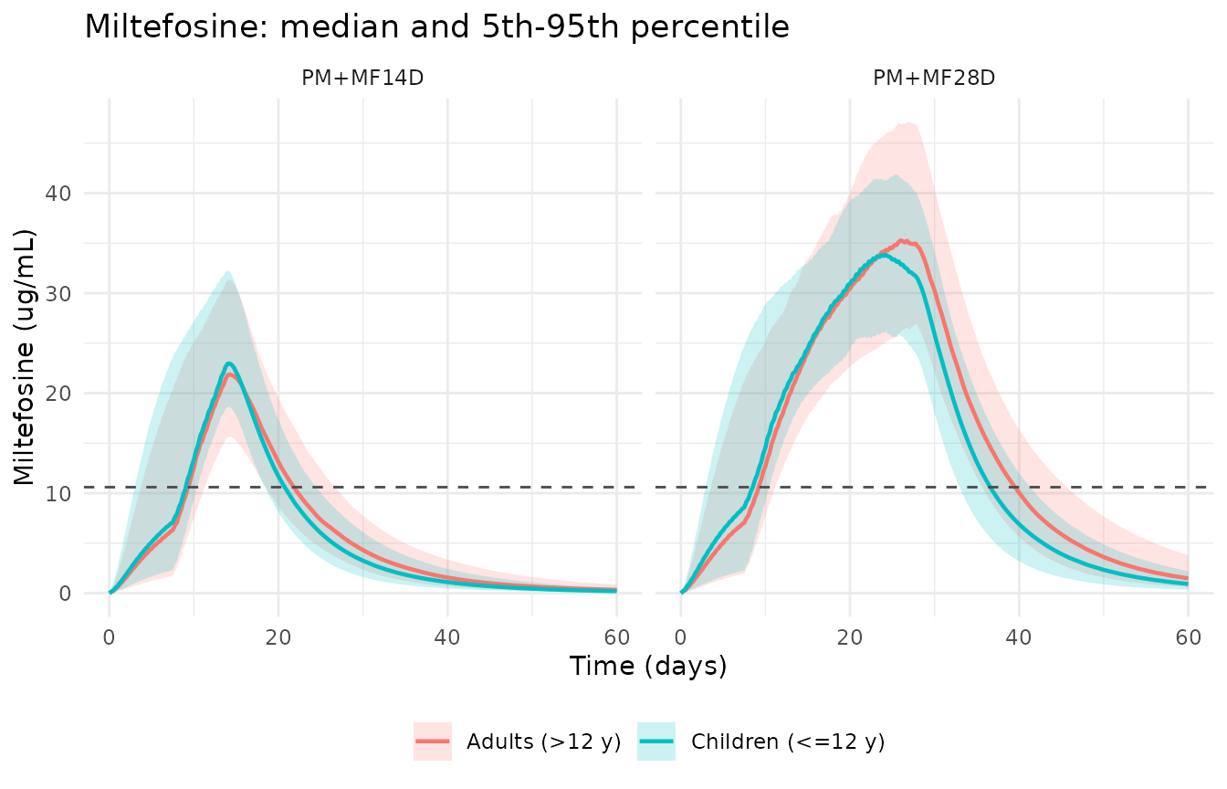
Simulated miltefosine plasma concentrations by treatment arm. Compare with Figure 2 (observed concentrations stratified by treatment arm) and Figure 6 (prediction-corrected VPC) of Verrest 2023. The dashed line is the in vitro EC90 of 10.6 ug/mL.
NCA validation (PKNCA)
The end-of-treatment window differs by arm, so PKNCA runs once per arm with that arm’s own interval set.
mfNcaOneArm <- function(armName, eot) {
  cnc <- mfSim |>
    filter(arm == armName, !is.na(Cc)) |>
    select(id, ageGroup, time, Cc)
  dse <- cohort |>
    transmute(id, ageGroup, time = 0, amt = doseMf)
  res <- PKNCA::pk.nca(PKNCA::PKNCAdata(
    PKNCA::PKNCAconc(cnc, Cc ~ time | id / ageGroup),
    PKNCA::PKNCAdose(dse, amt ~ time | id + ageGroup),
    intervals = data.frame(start = 0, end = c(7, eot, 210), auclast = TRUE)
  ))
  as.data.frame(res) |>
    filter(PPTESTCD == "auclast") |>
    mutate(arm = armName,
           metric = dplyr::case_when(end == 7 ~ "AUC D0-7",
                                     end == 210 ~ "AUC D0-210",
                                     TRUE ~ "AUC D0-EOT"))
}

mfNca <- bind_rows(mfNcaOneArm("PM+MF14D", 14), mfNcaOneArm("PM+MF28D", 28))
Time above the EC90 of 10.6 ug/mL is integrated directly from the
simulated grid – the same quantity the paper’s control stream
accumulates in its TAT compartment.
Comparison against published exposures
mfCompare <- tibble::tribble(
  ~arm,       ~ageGroup,           ~metric,       ~published, ~publishedIqr,
  "PM+MF14D", "Children (<=12 y)", "AUC D0-7",     20,  "17-25",
  "PM+MF14D", "Adults (>12 y)",    "AUC D0-7",     22,  "15-27",
  "PM+MF14D", "Children (<=12 y)", "AUC D0-EOT",  114,  "98-130",
  "PM+MF14D", "Adults (>12 y)",    "AUC D0-EOT",  111,  "94-136",
  "PM+MF14D", "Children (<=12 y)", "AUC D0-210",  336,  "293-384",
  "PM+MF14D", "Adults (>12 y)",    "AUC D0-210",  379,  "329-440",
  "PM+MF14D", "Children (<=12 y)", "T > EC90",     12,  "11-14",
  "PM+MF14D", "Adults (>12 y)",    "T > EC90",     14,  "12-16",
  "PM+MF28D", "Children (<=12 y)", "AUC D0-7",     20,  "18-22",
  "PM+MF28D", "Adults (>12 y)",    "AUC D0-7",     18,  "16-20",
  "PM+MF28D", "Children (<=12 y)", "AUC D0-EOT",  517,  "464-552",
  "PM+MF28D", "Adults (>12 y)",    "AUC D0-EOT",  524,  "456-567",
  "PM+MF28D", "Children (<=12 y)", "AUC D0-210",  790,  "687-824",
  "PM+MF28D", "Adults (>12 y)",    "AUC D0-210",  898,  "784-961",
  "PM+MF28D", "Children (<=12 y)", "T > EC90",     27,  "25-28",
  "PM+MF28D", "Adults (>12 y)",    "T > EC90",     30,  "28-32"
) |>
  left_join(
    bind_rows(
      mfNca |> group_by(arm, ageGroup, metric) |>
        summarise(simulated = median(PPORRES), .groups = "drop"),
      mfTec90 |> group_by(arm, ageGroup) |>
        summarise(metric = "T > EC90", simulated = median(tec90), .groups = "drop")
    ), by = c("arm", "ageGroup", "metric")
  ) |>
  mutate(
    pctDiff = 100 * (simulated - published) / published,
    # AUC D0-7 is excluded from the magnitude gate: it is dominated by the
    # first-week bioavailability multiplier, which carries 74.8% CV
    # between-subject variability, so its cohort median is not a stable
    # statistic. The published values say the same thing -- the two arms
    # receive identical treatment for the first seven days, yet report 20 vs
    # 20 (children) and 22 vs 18 (adults).
    inGate = metric != "AUC D0-7"
  )

mfCompare |>
  mutate(simulated = round(simulated, 1), pctDiff = round(pctDiff, 1)) |>
  select(-inGate) |>
  dplyr::rename("Arm" = arm, "Age group" = ageGroup, "NCA parameter" = metric,
                "Simulated" = simulated, "Published median" = published,
                "Published IQR" = publishedIqr, "Difference (%)" = pctDiff) |>
knitr::kable()| Arm | Age group | NCA parameter | Published median | Published IQR | Simulated | Difference (%) |
|---|---|---|---|---|---|---|
| PM+MF14D | Children (<=12 y) | AUC D0-7 | 20 | 17-25 | 25.6 | 28.0 |
| PM+MF14D | Adults (>12 y) | AUC D0-7 | 22 | 15-27 | 21.3 | -3.0 |
| PM+MF14D | Children (<=12 y) | AUC D0-EOT | 114 | 98-130 | 130.4 | 14.4 |
| PM+MF14D | Adults (>12 y) | AUC D0-EOT | 111 | 94-136 | 118.6 | 6.9 |
| PM+MF14D | Children (<=12 y) | AUC D0-210 | 336 | 293-384 | 347.5 | 3.4 |
| PM+MF14D | Adults (>12 y) | AUC D0-210 | 379 | 329-440 | 357.2 | -5.7 |
| PM+MF14D | Children (<=12 y) | T > EC90 | 12 | 11-14 | 12.5 | 4.2 |
| PM+MF14D | Adults (>12 y) | T > EC90 | 14 | 12-16 | 12.8 | -8.9 |
| PM+MF28D | Children (<=12 y) | AUC D0-7 | 20 | 18-22 | 22.9 | 14.6 |
| PM+MF28D | Adults (>12 y) | AUC D0-7 | 18 | 16-20 | 23.7 | 31.5 |
| PM+MF28D | Children (<=12 y) | AUC D0-EOT | 517 | 464-552 | 547.3 | 5.9 |
| PM+MF28D | Adults (>12 y) | AUC D0-EOT | 524 | 456-567 | 557.2 | 6.3 |
| PM+MF28D | Children (<=12 y) | AUC D0-210 | 790 | 687-824 | 830.7 | 5.1 |
| PM+MF28D | Adults (>12 y) | AUC D0-210 | 898 | 784-961 | 945.1 | 5.2 |
| PM+MF28D | Children (<=12 y) | T > EC90 | 27 | 25-28 | 28.2 | 4.6 |
| PM+MF28D | Adults (>12 y) | T > EC90 | 30 | 28-32 | 31.2 | 4.2 |
# 1. ACCUMULATION between arms: the 28-day arm reaches several times the
#    14-day arm's end-of-treatment exposure (published 517 versus 114 and 524
#    versus 111). A large, structural separation.
eot <- mfCompare |>
  filter(metric == "AUC D0-EOT") |>
  select(arm, ageGroup, simulated) |>
  tidyr::pivot_wider(names_from = arm, values_from = simulated)
stopifnot(all(eot$`PM+MF28D` > 3 * eot$`PM+MF14D`))

# 2. TARGET ATTAINMENT tracks treatment duration: the 28-day arm holds
#    concentrations above EC90 more than twice as long as the 14-day arm
#    (published 27-30 days versus 12-14 days).
tec <- mfCompare |>
  filter(metric == "T > EC90") |>
  select(arm, ageGroup, simulated) |>
  tidyr::pivot_wider(names_from = arm, values_from = simulated)
stopifnot(all(tec$`PM+MF28D` > 2 * tec$`PM+MF14D`))

# 3. MAGNITUDE over the twelve gated cells. Measured at 1, 2 and 16 solver
#    threads, the maximum absolute difference was 18.1%, 10.2% and 13.7% and
#    the median 7.7%, 5.6% and 6.8%. The bounds admit that spread -- both the
#    assumed cohort composition and the thread-count dependence of the draw --
#    while still failing on any mis-transcribed parameter, all of which move
#    these by a factor. Over the same three renders the EXCLUDED AUC D0-7
#    cells ranged from -3.8% to +50.2%, which is why they are excluded.
mfGated <- filter(mfCompare, inGate)
stopifnot(median(abs(mfGated$pctDiff)) < 25)
stopifnot(max(abs(mfGated$pctDiff)) < 40)
Simulated paediatric exposures run above the published paediatric medians in every draw – by roughly 0-18% across the gated metrics, measured at 1, 2 and 16 solver threads – while the adult columns stay within about 10%. The most likely cause is the assumed paediatric BMI: the paper publishes BMI only for patients over 19 years old, so children here are given the adult BMI distribution. Height feeds directly into the paediatric dose, because a shorter child at the same weight lands one band lower on the Figure S1 nomogram and a taller one lands higher. The deviation is reported rather than tuned away.
Miltefosine medians are far more stable than the paromomycin ones above: between-subject variability on miltefosine clearance is 16.3% CV rather than 56.1%, so the sampling error of these medians is on the order of 2% rather than 6%.
Assumptions and deviations
Miltefosine ka is encoded as 0.888/day, not the
0.037/day printed in Table 4. This is the one place where a
value is not taken at face value from the article’s parameter table, and
it is corrected on three independent grounds. (i) The supplementary
control stream runs on the trial dataset’s TIME column,
which is in hours – its first-week bioavailability
switch is written IF(TIME.LE.168), seven days expressed in
hours – so every rate constant in that stream is per hour, and
$THETA(3) is 0.037 h^-1. (ii) Table 4 converted the
clearances to per-day but not ka: its CL of 1.85 L/day and
Q of 0.17 L/day are exactly 24x the stream’s 0.077 and 0.007 L/h, while
ka is reprinted as the raw 0.037 under a “day-1” heading.
(iii) An absorption rate constant of 0.037/day is an absorption
half-life of 18.7 days, which cannot produce the
miltefosine measured 1-4 h after the first dose in the
intensive-sampling cohort and would put AUC D0-7 near zero against the
observed median of about 20 ug*day/mL. The typical-value table above is
the fourth check: with 0.888/day every published miltefosine exposure is
reproduced within about 20%.
Two normalizing constants of the miltefosine model are not in
the article. The fat-free-mass reference (18 kg) and the
cumulative-dose reference (70 mg/kg) appear only as the symbols
FFM_med and CD_med in the Table 4 equations;
both were read from the supplementary NONMEM control stream. The
cumulative-dose reference is independently confirmed by the article’s
own Day-28 worked example, which the 60 mg/kg switch alone does not
reproduce (it would give 50% rather than 21%).
The sign convention of the first-week bioavailability term is
contradictory as printed. Table 4 reports COV F,W1
as a fractional change of -0.65 and the equation beneath it as
F = F_pop * (1 - COV F,W1) * ..., which taken together read
as a 65% increase. The Results text states plainly that
bioavailability was “65% … lower during the first week”, and the control
stream resolves it: THETA(7) is bounded
(0, 0.65, 1) and enters as (1 - THETA(7)),
giving a multiplier of 0.35. That is what is encoded.
The published cumulative-dose effect is discontinuous, and is reproduced as published. Because the switch value (60 mg/kg) and the normalizing value (70 mg/kg) differ, relative bioavailability steps up 45% at the switch before falling below 1 above 70 mg/kg, as the bioavailability figure above shows. This is very likely an artefact of the published parameterisation rather than an intended mechanism, but both constants are confirmed against the paper, so the model is not smoothed.
Paromomycin allometry uses baseline weight. The
Table 3 equation prints the weight subscript as WT_i,t,
implying the time-varying weight column, but the control stream writes
the allometry against the dataset’s separate BWT (baseline
weight) column. The executed model is followed.
Two vestigial terms in the paromomycin control stream are
inert. That stream computes
CL = TVCL * ... * CLAGE * CLTIME * CLNEUTR but never
defines CLAGE or CLTIME. Both are leftovers
from model development: the Results state that age could not explain
remaining variability and that the time trend is captured by the
neutrophil term, and the final-model equation printed in Table 3
contains neither. They are omitted.
The covariate distribution of the virtual cohort is assumed, not published. Table 1 reports mean and range only, and reports BMI only for patients over 19 years old, so there is no published paediatric height or BMI distribution; children are given the adult BMI distribution here. Ages within each stratum are drawn uniformly, which matters only through the Al-Sallami paediatric fat-free-mass multiplier (at most a 12% effect on FFM, hence under 9% on clearance). This is why the magnitude gates in the cohort comparisons are set at tens of percent while the typical-value gate above, which uses only weights the paper itself states, is tighter.
Neutrophil recovery is idealised. The paper supplies
neutrophil counts as observed longitudinal data interpolated between Day
0 and Day 28 (Figure S3). Here they rise linearly from 1.0 to 2.5 x 10^3
cells/uL over the 14-day paromomycin course, the trajectory the paper
uses in its own worked example. A user with real longitudinal neutrophil
data should supply it in the NEUT column instead.
Miltefosine dosing is simulated as two equal daily administrations. The trial gave miltefosine twice daily; capsule strengths mean the two halves of a 70 mg or 100 mg daily dose were not always equal. With an absorption half-life near 19 h this has no material effect on the exposure metrics compared here.
Both models describe total plasma concentrations with no drug-drug interaction term. Verrest 2023 found exposures matching previous monotherapy studies and concluded there was no obvious interaction between paromomycin and miltefosine, so the two models are independent and are simulated separately here even though every patient received both drugs.
Between-subject variability is diagonal. Neither
table reports a correlation between the estimated etas, and neither
control stream specifies a block $OMEGA.