Amikacin liposome inhalation suspension (Rubino 2021)
Source:vignettes/articles/Rubino_2021_amikacin.Rmd
Rubino_2021_amikacin.RmdModel and source
- Citation: Rubino CM, Onufrak NJ, van Ingen J, Griffith DE, Bhavnani SM, Yuen DW, Mange KC, Winthrop KL. Population Pharmacokinetic Evaluation of Amikacin Liposome Inhalation Suspension in Patients with Treatment-Refractory Nontuberculous Mycobacterial Lung Disease. Eur J Drug Metab Pharmacokinet. 2021;46(2):277-287. doi:10.1007/s13318-020-00669-7. Correction: Eur J Drug Metab Pharmacokinet. 2021. doi:10.1007/s13318-021-00687-z (corrects the Figure 2 x-axis labels and a figure cross-reference only; no model value is affected). The structural model, zero-order lung input and additive residual-error form are carried from the cystic fibrosis model it was based on: Okusanya OO, Bhavnani SM, Hammel JP, Forrest A, Bulik CC, Ambrose PG, Gupta R. Antimicrob Agents Chemother. 2014;58(9):5005-5015. doi:10.1128/AAC.02421-13.
- Description: One-compartment population PK model for amikacin in serum after once-daily nebulised amikacin liposome inhalation suspension (ALIS) 590 mg in adults with treatment-refractory nontuberculous mycobacterial (NTM) lung disease (Rubino 2021). Zero-order nebulised input into a lung absorption compartment, first-order absorption from lung to serum, and linear apparent clearance CLt/F from an apparent central volume Vc/F; a urine compartment accumulates the renally excreted amount at the true renal clearance CLr (allometrically scaled by body weight to a 51 kg reference), so the serum concentration and the cumulative urine amount were fit simultaneously and the systemic bioavailability is implied by CLr / (CLt/F).
- Article: https://doi.org/10.1007/s13318-020-00669-7
- Correction (Figure 2 axis labels only): https://doi.org/10.1007/s13318-021-00687-z
- Base model (cystic fibrosis, Okusanya 2014): https://doi.org/10.1128/AAC.02421-13
Amikacin liposome inhalation suspension (ALIS, ARIKAYCE) is nebulised once daily at 590 mg. Rubino 2021 pooled the serum (and, in TR02-112, urine) data of the phase 2 TR02-112 and phase 3 CONVERT pharmacokinetic substudies and refit the model previously developed in cystic fibrosis (Okusanya 2014) without changing its structure: a zero-order nebulised input into a lung absorption compartment, first-order transfer to serum, linear elimination at the apparent clearance CLt/F, and a urine compartment that accumulates the renally excreted amount at the renal clearance CLr (Figure 1). Because CLt/F and Vc/F are apparent while CLr is fitted to urine amounts, the ratio CLr / (CLt/F) is the fraction of the nebulised dose that is recovered unchanged in urine, i.e. the systemic bioavailability for a drug that is cleared almost entirely by the kidney.
Population
The analysis population (Table 1) comprised 53 adults with treatment-refractory nontuberculous mycobacterial (NTM) lung disease: 14 from TR02-112 (all White, all female; USA and Canada) and 39 from CONVERT (28 Japanese and 11 White; USA and Japan). The median age was 63 years (range 20-84), 84.9% were female, the median body weight was 52.6 kg (33.8-80 kg), and the median eGFR was 88.3 mL/min/1.73 m^2 (57.4-140). Sputum was persistently culture-positive for Mycobacterium avium complex (both studies) or M. abscessus (TR02-112) after at least 6 months of guideline-based therapy. 491 serum concentrations (89 below the 0.15 mg/L LLOQ, handled by the Beal M3 method) and 23 urine collections (TR02-112 only) were analysed.
The same information is available programmatically via
readModelDb("Rubino_2021_amikacin")()$population.
Source trace
| Equation / parameter | Value | Source location |
|---|---|---|
lcl (CLt/F) |
34.29 L/h | Table 2 |
lvc (Vc/F) |
272.6 L | Table 2 |
lka (ka) |
1.866 1/h | Table 2 |
lcl_renal (CLr at 51 kg) |
1.931 L/h | Table 2, ‘CLr coefficient’ and footnote |
e_wt_cl_renal |
0.75 (fixed) | Table 2, ‘CLr WTKG power’ (no %SEM) and footnote equation |
etalcl |
71.82 %CV | Table 2 |
etalvc |
65.09 %CV | Table 2 |
etalka |
40.30 %CV | Table 2 |
etalcl_renal |
30.24 %CV | Table 2 |
addSd (serum) |
0.615 mg/L | Table 2, ‘Residual error (serum)’; additive form from Methods 2.3 and Okusanya 2014 |
addSd_Aurine (urine) |
14.0 mg | Table 2, ‘Residual error (urine)’; additive form as above |
CLr = 1.931 * (WT/51)^0.75 |
n/a | Table 2 footnote |
| Lung -> serum -> urine structure, zero-order lung input | n/a | Figure 1; Methods 2.3 |
d/dt(urine) = CLr * Cc |
n/a | Methods 2.3 (‘Amikacin in urine was modeled as accumulating in the urine compartment after clearance from the central compartment’) |
Table 2 also lists ‘CLr = 1.990 L/h’ with no standard error. It is the population mean renal clearance across the analysed patients implied by the weight equation (1.931 x (WT/51)^0.75 evaluated at a weight near the cohort mean), not a separate parameter, so it is not encoded.
Structural checks (typical patient, 51 kg)
mod <- readModelDb("Rubino_2021_amikacin")
mod_typ <- rxode2::zeroRe(mod)
#> ℹ parameter labels from comments will be replaced by 'label()'

dose <- 590
tau <- 24
n_days <- 168
t_ss <- (n_days - 1) * tau

ev_typ <- rxode2::et(amt = dose, cmt = "depot", dur = 0.25, ii = tau, addl = n_days - 1) |>
  rxode2::et(c(seq(0, 24, by = 0.02), seq(t_ss, t_ss + tau, by = 0.02)), cmt = "central") |>
  as.data.frame() |>
  mutate(WT = 51, dvid = ifelse(evid == 0, 1L, NA_integer_))

typ <- rxode2::rxSolve(mod_typ, ev_typ,
  useLinCmt = FALSE, returnType = "data.frame",
  rtol = 1e-10, atol = 1e-12, maxsteps = 1e6
)
#> ℹ omega/sigma items treated as zero: 'etalcl', 'etalvc', 'etalka', 'etalcl_renal'

trap <- function(t, y) sum(diff(t) * (head(y, -1) + tail(y, -1)) / 2)
typ_ss <- typ |> filter(time >= t_ss)
typ_d1 <- typ |> filter(time <= tau)

auc_ss <- trap(typ_ss$time, typ_ss$Cc)
fe_ss <- (max(typ_ss$Aurine) - min(typ_ss$Aurine)) / dose
thalf <- log(2) * 272.6 / 34.29

typ_tab <- tibble::tribble(
  ~Quantity, ~Simulated, ~Expected,
  "AUC0-24 at steady state (mg*h/L)", auc_ss, dose / 34.29,
  "Fraction of dose in urine per interval at steady state (%)", 100 * fe_ss, 100 * 1.931 / 34.29,
  "Cmax day 1 (mg/L)", max(typ_d1$Cc), NA,
  "Cmax steady state (mg/L)", max(typ_ss$Cc), NA,
  "AUC0-24 day 1 (mg*h/L)", trap(typ_d1$time, typ_d1$Cc), NA,
  "Elimination half-life ln2*Vc/CL (h)", thalf, 5.48
)
knitr::kable(typ_tab, digits = 3, caption = paste(
  "Typical-value checks. The steady-state rows are closed-form identities",
  "(AUC = Dose/(CLt/F); urine recovery = CLr/(CLt/F)); the half-life row compares",
  "with the median post hoc half-life of Table 3."
))| Quantity | Simulated | Expected |
|---|---|---|
| AUC0-24 at steady state (mg*h/L) | 17.206 | 17.206 |
| Fraction of dose in urine per interval at steady state (%) | 5.631 | 5.631 |
| Cmax day 1 (mg/L) | 1.780 | NA |
| Cmax steady state (mg/L) | 1.878 | NA |
| AUC0-24 day 1 (mg*h/L) | 16.291 | NA |
| Elimination half-life ln2*Vc/CL (h) | 5.510 | 5.480 |
stopifnot(
  # Closed-form identities: both sides use the same parameters, so the only
  # difference is integration error (measured ~1e-7 with the tolerances above).
  abs(auc_ss / (dose / 34.29) - 1) < 1e-4,
  abs(fe_ss / (1.931 / 34.29) - 1) < 1e-4,
  # Typical half-life vs the Table 3 median of the post hoc half-lives (5.48 h).
  abs(thalf / 5.48 - 1) < 0.02
)
The implied systemic bioavailability, CLr / (CLt/F) =
1.931 / 34.29 = 5.6% for a 51 kg patient, agrees with the paper’s
conclusion that less than 10% of the nebulised dose reaches the systemic
circulation.
Virtual cohort
Observed data are not public. The cohort below draws body weight from a log-normal distribution centred on the Table 1 median (52.6 kg) and rejects draws outside the observed 33.8-80 kg range (redrawing, not clamping, so the weight distribution is not piled up at the limits). Weight is the only covariate in the model. All patients receive ALIS 590 mg once daily for 168 days (the approximately 6-month time point of Table 3).
set.seed(20210301)
n_sub <- 200

draw_wt <- function(n) {
  out <- numeric(0)
  while (length(out) < n) {
    x <- exp(rnorm(2 * n, log(52.6), 0.2))
    out <- c(out, x[x >= 33.8 & x <= 80])
  }
  out[seq_len(n)]
}

subj <- tibble(id = seq_len(n_sub), WT = draw_wt(n_sub))

obs_times <- c(seq(0, 24, by = 0.25), seq(t_ss, t_ss + tau, by = 0.25))

events <- bind_rows(
  subj |> mutate(
    time = 0, amt = dose, evid = 1L, cmt = "depot", dur = 0.25,
    ii = tau, addl = n_days - 1L, dvid = NA_integer_
  ),
  tidyr::crossing(subj, time = obs_times) |> mutate(
    amt = NA_real_, evid = 0L, cmt = "central", dur = NA_real_,
    ii = NA_real_, addl = NA_integer_, dvid = 1L
  )
) |>
  arrange(id, time, desc(evid))

stopifnot(!anyDuplicated(events[, c("id", "time", "evid")]))
Simulation
rxode2::rxSetSeed(20210301)
sim <- rxode2::rxSolve(mod, events,
  keep = "WT", useLinCmt = FALSE,
  returnType = "data.frame", maxsteps = 1e6
)
#> ℹ parameter labels from comments will be replaced by 'label()'

# Concentration and cumulative-urine predictions without residual error,
# separated into the day-1 and day-168 dosing intervals and re-based to time
# after dose.
sim_int <- sim |>
  filter(time <= tau | time >= t_ss) |>
  mutate(
    period = ifelse(time <= tau, "Day 1", "Day 168"),
    tad = ifelse(period == "Day 1", time, time - t_ss)
  )
Replicate published figures
Figure 2 of the paper plots the observed serum concentrations against time since the last dose. The simulated median and 90% prediction interval of the individual predictions over one dosing interval on day 1 and on day 168 cover the same range: peaks around 1-6 mg/L within the first few hours and troughs near or below the 0.15 mg/L LLOQ by 24 h.
sim_int |>
  group_by(period, tad) |>
  summarise(
    Q05 = quantile(Cc, 0.05), Q50 = median(Cc), Q95 = quantile(Cc, 0.95),
    .groups = "drop"
  ) |>
  ggplot(aes(tad, Q50, colour = period, fill = period)) +
  geom_ribbon(aes(ymin = Q05, ymax = Q95), alpha = 0.2, colour = NA) +
  geom_line() +
  geom_hline(yintercept = 0.15, linetype = "dashed") +
  scale_y_log10() +
  scale_x_continuous(breaks = seq(0, 24, 4)) +
  labs(
    x = "Time since last dose (h)", y = "Serum amikacin (mg/L)",
    colour = NULL, fill = NULL,
    caption = paste(
      "Compare with Figure 2 of Rubino 2021. Median and 90% prediction interval",
      "(no residual error); dashed line = 0.15 mg/L LLOQ."
    )
  )
#> Warning in scale_y_log10(): log-10 transformation introduced infinite values.
#> log-10 transformation introduced infinite values.
#> log-10 transformation introduced infinite values.
#> log-10 transformation introduced infinite values.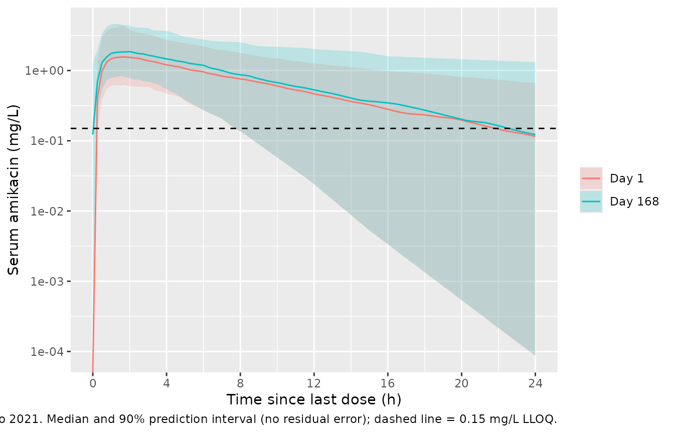
PKNCA validation
Table 3 of the paper reports the median model-derived Cmax and AUC0-24 on day 1 and at approximately 6 months (all 53 patients). PKNCA is run on each dosing interval of the virtual cohort with the period as the grouping variable.
sim_nca <- sim_int |>
  filter(!is.na(Cc)) |>
  select(id, period, tad, Cc)

# Day 1 starts at zero concentration; the day-168 interval has its own
# pre-dose (trough) record at tad = 0 from the observation grid.
sim_nca <- bind_rows(
  sim_nca,
  sim_nca |> distinct(id, period) |> filter(period == "Day 1") |> mutate(tad = 0, Cc = 0)
) |>
  distinct(id, period, tad, .keep_all = TRUE) |>
  arrange(id, period, tad)

dose_df <- sim_nca |>
  distinct(id, period) |>
  mutate(tad = 0, amt = dose)

conc_obj <- PKNCA::PKNCAconc(sim_nca, Cc ~ tad | period + id, concu = "mg/L", timeu = "h")
dose_obj <- PKNCA::PKNCAdose(dose_df, amt ~ tad | period + id, doseu = "mg")
intervals <- data.frame(start = 0, end = 24, cmax = TRUE, tmax = TRUE, auclast = TRUE)
nca_res <- PKNCA::pk.nca(PKNCA::PKNCAdata(conc_obj, dose_obj, intervals = intervals))
Comparison against published NCA
published <- tibble::tribble(
  ~period, ~cmax, ~auclast,
  "Day 1", 1.70, 15.8,
  "Day 168", 1.81, 16.7
)

cmp <- nlmixr2lib::ncaComparisonTable(
  simulated = nca_res,
  reference = published,
  by = "period",
  units = c(cmax = "mg/L", auclast = "mg*h/L"),
  tolerance_pct = 20
)
knitr::kable(cmp, caption = paste(
  "Median simulated vs. published (Rubino 2021 Table 3, total N = 53) Cmax and",
  "AUC0-24. Day 168 corresponds to the paper's approximately 6-month column.",
  "* differs from reference by >20%."
))| NCA parameter | period | Reference | Simulated | % diff |
|---|---|---|---|---|
| Cmax (mg/L) | Day 1 | 1.7 | 1.63 | -4.4% |
| Cmax (mg/L) | Day 168 | 1.81 | 1.89 | +4.7% |
| AUClast (mg*h/L) | Day 1 | 15.8 | 15.7 | -0.4% |
| AUClast (mg*h/L) | Day 168 | 16.7 | 17.5 | +5.1% |
sim_med <- as.data.frame(nca_res$result) |>
  filter(PPTESTCD %in% c("cmax", "auclast")) |>
  group_by(period, PPTESTCD) |>
  summarise(med = median(PPORRES), .groups = "drop") |>
  left_join(
    published |> pivot_longer(-period, names_to = "PPTESTCD", values_to = "ref"),
    by = c("period", "PPTESTCD")
  )
stopifnot(
  nrow(sim_med) == 4L,
  # Cohort medians: a mis-transcribed CL, V or dose moves these by tens of
  # percent. The steady-state AUC median is Dose / median(CLt/F) and is
  # almost cohort-independent; the others carry sampling noise of a few percent.
  all(abs(sim_med$med / sim_med$ref - 1) < 0.15)
)
The simulated medians reproduce the published medians closely. The paper’s values are medians of the empirical Bayes estimates of the 53 analysed patients, which are shrunk towards the typical value, so the published ranges (Cmax 0.465-6.87 mg/L, AUC0-24 4.16-55.6 mg*h/L) are expected to be narrower than a simulated cohort’s tails; only the centres are compared.
Urinary recovery
Table S2 of the paper reports the percentage of the dose excreted unchanged in urine over the 24 h after the day-1, day-84 and day-168 doses in TR02-112 (White women, median weight 65.2 kg).
fe <- sim_int |>
  group_by(id, period) |>
  summarise(fe_pct = 100 * (max(Aurine) - min(Aurine)) / dose, .groups = "drop")

fe_tab <- fe |>
  group_by(period) |>
  summarise(
    "Simulated median (%)" = median(fe_pct),
    "Simulated 5th-95th percentile (%)" = sprintf(
      "%.2f-%.2f", quantile(fe_pct, 0.05), quantile(fe_pct, 0.95)
    ),
    .groups = "drop"
  ) |>
  mutate(
    "Observed median, range (%)" = c("3.25 (2.71-8.95), n = 6", "8.42 (0.72-22.6), n = 11")
  ) |>
  rename(Period = period)
knitr::kable(fe_tab, digits = 2, caption = paste(
  "Percentage of the 590 mg dose excreted unchanged in urine over 24 h.",
  "Observed values from Rubino 2021 Table S2 (TR02-112)."
))| Period | Simulated median (%) | Simulated 5th-95th percentile (%) | Observed median, range (%) |
|---|---|---|---|
| Day 1 | 5.08 | 1.71-13.88 | 3.25 (2.71-8.95), n = 6 |
| Day 168 | 5.88 | 1.83-19.54 | 8.42 (0.72-22.6), n = 11 |
stopifnot(
  # The model has no time dependency, so both intervals centre on
  # CLr / (CLt/F); the centre must sit inside the observed day-1 to day-168
  # spread of medians (3.25-8.42%).
  all(tapply(fe$fe_pct, fe$period, median) > 3.25),
  all(tapply(fe$fe_pct, fe$period, median) < 8.42)
)
The observed median recovery rose from 3.25% on day 1 to 8.42% on day 168 in the small TR02-112 urine subset, while the model (which has no time-varying bioavailability) places both intervals at about 5-6%, between the two observed medians; the paper also reports the model-derived exposure as differing by less than 10% between day 1 and 6 months.
Assumptions and deviations
-
IIV scale. Table 2 reports inter-individual
variability as %CV of an exponential (log-normal) model without stating
the back-transformation. The variances were computed as
omega^2 = log(CV^2 + 1); the alternative readingomega = CVwould give variances of 0.516, 0.424, 0.162 and 0.091 (instead of 0.416, 0.353, 0.150 and 0.088) for CLt/F, Vc/F, ka and CLr. No published quantity discriminates between them (the Table 3 ranges come from shrunk post hoc estimates). - Residual error form. Table 2 gives one residual-error value for serum (0.615) and one for urine (14.0) without naming the model. Methods 2.3 states that residual variability was initially described with an additive model and that separate models were used for serum and urine, and the cystic fibrosis model on which this analysis is based used separate additive error models for serum and urine (Okusanya 2014, Methods). The values are therefore encoded as additive standard deviations in mg/L (serum) and mg (urine amount).
-
Apparent frame. CLt/F and Vc/F are apparent
parameters and the full nebulised dose enters the lung compartment
(bioavailability is not a separate parameter). The urine compartment is
filled at the true renal clearance CLr times the serum concentration and
is not subtracted from the central compartment, whose total loss is
already CLt/F (dotted arrow in Figure 1). Individual bioavailability is
therefore
CLr / (CLt/F)under the assumption, standard for amikacin, that elimination is almost entirely renal. -
Urine collections. The paper collected urine over
0-24 h after the dose; the Okusanya 2014 base model emptied the urine
compartment at the end of each collection interval. The packaged
urinestate is cumulative from the start of the simulation, so the amount over a collection interval is the difference inAurineacross it (as done above) or the state must be reset in the event table. - Nebulisation duration. The analysis used each patient’s recorded nebulisation start and end times. The simulations here use a 15-minute zero-order input; Okusanya 2014 reports 2-5 minutes per 140 mg (about 8-21 minutes for 590 mg). With ka = 1.87 1/h the duration has little effect on Cmax or AUC.
- Race. Japanese and White patients had similar exposures and the model has no race covariate; the virtual cohort is described by weight only.
- Inter-occasion variability was not estimated (Methods 2.3), and sputum concentrations were not modelled, so neither is part of this model.