Model and source
- Citation: Ji E, Kim MG, Oh JM. CYP3A5 genotype-based model to predict tacrolimus dosage in the early postoperative period after living donor liver transplantation. Ther Clin Risk Manag. 2018;14:2119-2126. doi:10.2147/TCRM.S184376
- Description: One-compartment population pharmacokinetic model for oral tacrolimus in Korean adult living-donor liver-transplant recipients during the first 14 days post-transplantation (Ji 2018). First-order absorption with ka fixed at 4.48 1/h from prior reports; CL/F = 6.33 * POD^0.257 multiplied by a combinational CYP3A5 recipient-and-donor categorical factor (2.314 if both recipient and donor are CYP3A5 expressers; 1.523 if the recipient is a CYP3A5 expresser and the donor is a nonexpresser; 1.0 otherwise); V/F = 465 * POD^0.322; exponential IIV on CL/F and V/F; combined proportional + additive residual error on whole-blood tacrolimus concentration.
- Article: https://doi.org/10.2147/TCRM.S184376
Population
The model was developed from 605 whole-blood tacrolimus trough concentrations collected over the first 14 days post-transplantation from 58 Korean adult patients receiving de novo living-donor liver transplantation (LDLT) at Seoul National University Hospital (Ji 2018 Table 1). Mean age was 49.2 years (range 19-65), mean body weight 61.4 kg (range 40.1-85.5), and 79.3% of subjects were male. Patients received oral tacrolimus (Astellas Prograf) twice daily at 10:00 and 22:00 on an empty stomach, starting on postoperative day 1; per-dose range was 0.1-6 mg (mean 1.9 mg). Doses were adjusted by therapeutic drug monitoring to a whole-blood trough target of 8-13 ng/mL for the triple-drug regimen (tacrolimus + corticosteroid + mycophenolate mofetil) or 13-17 ng/mL for the double-drug regimen (tacrolimus + corticosteroid). Concomitant medications were corticosteroids in all patients and mycophenolate mofetil in a subset.
CYP3A5 expresser status was determined for both the graft recipient and the graft donor by mismatch PCR-RFLP at rs776746 (CYP3A5*3). Both the recipient and donor genotype distributions were in Hardy-Weinberg equilibrium. Patients were classified into four combinational groups: REDE (recipient expresser + donor expresser, n = 10), REDN (recipient expresser + donor nonexpresser, n = 13), RNDE (recipient nonexpresser + donor expresser, n = 8), and RNDN (recipient nonexpresser + donor nonexpresser, n = 27). Ji 2018 found similar estimated CL/F factors for RNDE and RNDN and pooled them into a single reference category (the model retains REDE and REDN as the only non-reference levels).
The same information is available programmatically via
readModelDb("Ji_2018_tacrolimus")$population after the
model is loaded.
Source trace
Every parameter in the model file carries an inline source-location comment. The table below collects the entries in one place.
| Equation / parameter | Value | Source location |
|---|---|---|
lka (ka, fixed) |
4.48 1/h | Methods + Table 2; literature value from references 14, 15 |
lcl (CL/F at POD = 1, recipient nonexpresser) |
6.33 L/h | Table 2, CL/F row (RSE 16%, bootstrap 4.48-8.06) |
lvc (V/F at POD = 1) |
465 L | Table 2, V/F row (RSE 11%, bootstrap 384-560) |
e_pod_cl (POD power exponent on CL/F) |
0.257 | Table 2, POD on CL/F row (RSE 30%, bootstrap 0.141-0.411) |
e_pod_vc (POD power exponent on V/F) |
0.322 | Table 2, POD on V/F row (RSE 16%, bootstrap 0.233-0.409) |
e_rede_cl (REDE multiplicative factor on CL/F) |
2.314 | Table 2, CYP3A5 genotype REDE row (RSE 12%, bootstrap 1.907-2.742) |
e_redn_cl (REDN multiplicative factor on CL/F) |
1.523 | Table 2, CYP3A5 genotype REDN row (RSE 32%, bootstrap 1.201-1.923) |
| IIV CL/F (omega^2 = 0.117) | IIV 34.2% | Table 2, omega^2 Cl/F row (RSE 23%, bootstrap 0.071-0.160) |
| IIV V/F (omega^2 = 0.207) | IIV 45.5% | Table 2, omega^2 V/F row (RSE 23%, bootstrap 0.139-0.289) |
| Proportional residual (sigma^2 = 0.182 -> SD 0.4266) | 42.7% | Table 2, sigma^2 proportional row (RSE 9%, bootstrap 0.151-0.203) |
| Additive residual (sigma^2 = 0.838 ng2/mL2 -> SD 0.9154 ng/mL) | 0.838 | Table 2, sigma^2 additive row (RSE 22%, bootstrap 0.509-1.156) |
| Final-model equation for CL/F | – | Results: “CL/F = 6.33 x POD^0.257 x 2.314 (REDE) x 1.523 (REDN)” |
| Final-model equation for V/F | – | Results: “V/F = 465 x POD^0.322” |
| One-compartment oral structure | – | Methods: “the one-compartmental model was selected by comparing the one-compartmental model and two-compartmental model according to the Akaike information criterion” |
| ka held fixed at 4.48 1/h | – | Methods: “Because the measured concentrations were C_trough, it was difficult to estimate the absorption phase. Thus, the absorption rate constant (k_a) was fixed at a value of 4.48 h^-1 based on previously published reports” |
Virtual cohort
The published dataset is not openly available, so the virtual cohorts
below mirror the demographics in Ji 2018 Table 1 and the combinational
CYP3A5 group distribution in Methods (REDE n = 10, REDN n = 13, RNDE n =
8, RNDN n = 27 from the n = 58 study population). Subject IDs are kept
disjoint across cohorts so the per-group simulations can be combined
with bind_rows without collisions.
set.seed(20180101)

n_per_geno <- 100L

make_cohort <- function(n, recip, donor, label, id_offset = 0L) {
  tibble(
    id                = id_offset + seq_len(n),
    WT                = pmin(pmax(rnorm(n, mean = 61.4, sd = 10.1), 40.1), 85.5),
    CYP3A5_EXPR       = recip,
    CYP3A5_EXPR_DONOR = donor,
    cohort            = label
  )
}

# Four combinational genotype cohorts.
demo <- bind_rows(
  make_cohort(n_per_geno, recip = 1L, donor = 1L, label = "REDE",
              id_offset =                 0L),
  make_cohort(n_per_geno, recip = 1L, donor = 0L, label = "REDN",
              id_offset =   n_per_geno),
  make_cohort(n_per_geno, recip = 0L, donor = 1L, label = "RNDE",
              id_offset = 2*n_per_geno),
  make_cohort(n_per_geno, recip = 0L, donor = 0L, label = "RNDN",
              id_offset = 3*n_per_geno)
) |>
  mutate(cohort = factor(cohort, levels = c("REDE", "REDN", "RNDE", "RNDN")))
stopifnot(!anyDuplicated(demo$id))
Simulation
Two simulation scenarios are used:
- Typical-value CL/F and V/F vs POD (no IIV, no residual error) to reproduce Ji 2018 Figures 1B and 2.
- q12h oral dosing for 14 days with population IIV to characterise the trough distribution and to compare against the dose-suggestion table (Ji 2018 Table 3).
mod         <- rxode2::rxode2(readModelDb("Ji_2018_tacrolimus"))
#> ℹ parameter labels from comments will be replaced by 'label()'
mod_typical <- rxode2::zeroRe(mod)
Scenario 1 – typical-value CL/F and V/F across POD 1-14
# Time grid: probe POD = 1 .. 14 directly by simulating once per
# combinational group with no doses (the d/dt(central) ODE is integrated
# only for cl and vc evaluation as functions of POD; we evaluate cl and
# vc at one observation per POD).
pod_grid <- 1:14

theta_values <- tibble::tibble(
  cohort      = factor(c("REDE", "REDN", "RNDE", "RNDN"),
                       levels = c("REDE", "REDN", "RNDE", "RNDN")),
  CYP3A5_EXPR       = c(1L, 1L, 0L, 0L),
  CYP3A5_EXPR_DONOR = c(1L, 0L, 1L, 0L),
  cyp_factor        = c(2.314, 1.523, 1.000, 1.000)
)

theta_curve <- tidyr::expand_grid(
  cohort = factor(c("REDE", "REDN", "RNDE", "RNDN"),
                  levels = c("REDE", "REDN", "RNDE", "RNDN")),
  POD    = pod_grid
) |>
  dplyr::left_join(theta_values, by = "cohort") |>
  mutate(cl_typ = 6.33 * POD^0.257 * cyp_factor,
         v_typ  = 465  * POD^0.322)
Scenario 2 – q12h dosing for 14 days
build_events <- function(demo, dose_mg = 2.0, n_days = 14, dense = FALSE) {
  n_doses <- 2 * n_days  # twice daily for n_days
  doses <- demo |>
    mutate(amt  = dose_mg, evid = 1L, cmt = "depot",
           ii   = 12, addl = n_doses - 1L, time = 0) |>
    select(id, time, amt, evid, cmt, ii, addl, cohort,
           CYP3A5_EXPR, CYP3A5_EXPR_DONOR)

  # Observation grid: one morning-trough observation per POD (12 h after the
  # prior 22:00 dose -> 12 h after the AM dose -> the next morning's
  # 10:00 trough corresponds to t = (POD-1)*24 + 12 in the simulated clock).
  # An optional dense grid (`dense = TRUE`) refines the first-day absorption
  # phase for users who want full concentration-time curves.
  trough_times <- (seq_len(n_days) - 1L) * 24 + 12
  obs_times <- if (dense) {
    sort(unique(c(seq(0, 24, by = 1.0), trough_times)))
  } else {
    trough_times
  }

  obs <- demo |>
    select(id, cohort, CYP3A5_EXPR, CYP3A5_EXPR_DONOR) |>
    tidyr::crossing(time = obs_times) |>
    mutate(amt = NA_real_, evid = 0L, cmt = NA_character_,
           ii = NA_real_, addl = NA_integer_)

  events <- bind_rows(doses, obs) |>
    arrange(id, time, desc(evid)) |>
    mutate(POD = pmax(1, ceiling(time / 24)))
  events
}

events <- build_events(demo, dose_mg = 2.0, n_days = 14)
sim    <- rxode2::rxSolve(mod, events = events,
                          keep = c("cohort"), nStud = 1) |> as.data.frame()
Replicate published figures
Figure 1B – typical CL/F across POD 1-14 by combinational CYP3A5 group
Ji 2018 Figure 1B shows the estimated typical CL/F across POD 1-14, with separate curves for each of the four CYP3A5 combinational groups. RNDE and RNDN overlap (the model’s reference); REDN sits above; REDE is highest.
ggplot(theta_curve, aes(POD, cl_typ, colour = cohort, shape = cohort)) +
  geom_line(linewidth = 0.7) +
  geom_point(size = 1.7) +
  scale_x_continuous(breaks = 1:14) +
  labs(x = "Postoperative day (POD)",
       y = "Typical CL/F (L/h)",
       colour = "CYP3A5 group", shape = "CYP3A5 group",
       title = "Typical CL/F vs POD by combinational CYP3A5 genotype",
       caption = "Replicates Figure 1B of Ji 2018.")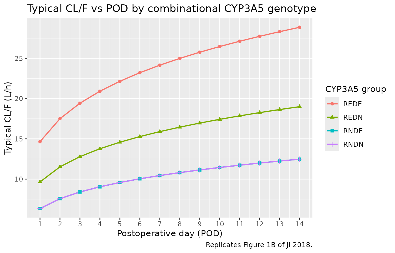
Replicates Figure 1B of Ji 2018: typical-value CL/F vs POD by combinational CYP3A5 genotype. CL/F = 6.33 x POD^0.257 x CYP3A5_factor.
Figure 2 – typical V/F across POD 1-14
Ji 2018 Figure 2 shows the typical V/F across POD 1-14 (no genotype effect on V/F).
theta_v <- tibble(POD = pod_grid) |>
  mutate(v_typ = 465 * POD^0.322)

ggplot(theta_v, aes(POD, v_typ)) +
  geom_line(linewidth = 0.7) +
  geom_point(size = 1.7) +
  scale_x_continuous(breaks = 1:14) +
  labs(x = "Postoperative day (POD)",
       y = "Typical V/F (L)",
       title = "Typical V/F vs POD",
       caption = "Replicates Figure 2 of Ji 2018.")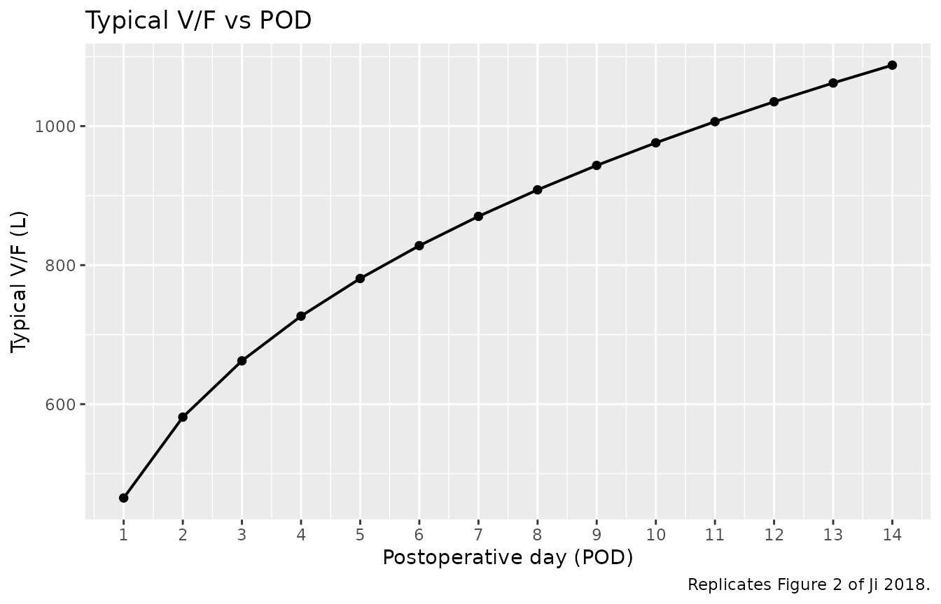
Replicates Figure 2 of Ji 2018: typical-value V/F vs POD. V/F = 465 x POD^0.322 (no CYP3A5 effect on V/F).
Figure 4 (analogue) – VPC of trough concentrations across POD 1-14
The published VPC (Ji 2018 Figure 4) plots observed and simulated concentrations across the first 14 days post-transplant. The vignette analogue below shows the simulated trough distribution per POD per combinational CYP3A5 group on a 2 mg q12h regimen.
trough_summary <- sim |>
  mutate(POD = pmax(1L, as.integer(ceiling(time / 24)))) |>
  group_by(POD, cohort) |>
  summarise(Q05 = quantile(Cc, 0.05),
            Q50 = quantile(Cc, 0.50),
            Q95 = quantile(Cc, 0.95),
            .groups = "drop")

ggplot(trough_summary, aes(POD, Q50, colour = cohort, fill = cohort)) +
  geom_ribbon(aes(ymin = Q05, ymax = Q95), alpha = 0.18, colour = NA) +
  geom_line(linewidth = 0.7) +
  geom_hline(yintercept = c(8, 13), linetype = "dashed", colour = "grey50") +
  scale_x_continuous(breaks = 1:14) +
  facet_wrap(~ cohort, ncol = 2) +
  labs(x = "Postoperative day (POD)",
       y = "Simulated trough Cc (ng/mL)",
       title = "Simulated trough distribution by CYP3A5 group on 2 mg BID",
       caption = "Dashed lines mark the 8-13 ng/mL triple-regimen trough target.") +
  theme(legend.position = "none")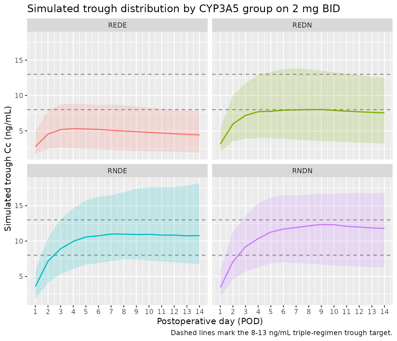
Simulated trough Cc (12 h after the prior 22:00 dose, i.e. ~10:00 the next morning) vs POD across the four combinational CYP3A5 groups on a 2 mg twice-daily regimen. The point ribbons summarise the 5th-95th percentile of the cohort at each POD. The cohort matches the n = 100 per-group virtual cohort built above.
PKNCA validation
NCA is run over the steady-state day-14 dosing interval (final dose at t = 13.5 days = 324 h, NCA window 324-336 h). The treatment grouping is the combinational CYP3A5 group.
# Re-simulate a small dense-sampled cohort over the day-14 dosing interval
# for NCA. The day-14 interval is treated as steady state (after 27 prior
# doses given q12h).
demo_nca <- demo |>
  group_by(cohort) |>
  slice_head(n = 25L) |>
  ungroup()

last_dose_time <- (14 - 1) * 24 + 12  # 324 h: noon on POD 14, the morning dose
nca_doses <- demo_nca |>
  mutate(amt = 2.0, evid = 1L, cmt = "depot", ii = 12, addl = 27L, time = 0,
         POD = 1L) |>
  select(id, time, amt, evid, cmt, ii, addl, cohort,
         CYP3A5_EXPR, CYP3A5_EXPR_DONOR, POD)
nca_obs <- demo_nca |>
  select(id, cohort, CYP3A5_EXPR, CYP3A5_EXPR_DONOR) |>
  tidyr::crossing(time = last_dose_time + seq(0, 12, by = 0.5)) |>
  mutate(amt = NA_real_, evid = 0L, cmt = NA_character_,
         ii = NA_real_, addl = NA_integer_,
         POD = pmax(1L, as.integer(ceiling(time / 24))))
events_nca <- bind_rows(nca_doses, nca_obs) |> arrange(id, time, desc(evid))

sim_nca_full <- rxode2::rxSolve(mod, events = events_nca,
                                keep = c("cohort"), nStud = 1) |> as.data.frame()

nca_window <- sim_nca_full |>
  filter(time >= last_dose_time, time <= last_dose_time + 12) |>
  mutate(time_after_dose = time - last_dose_time) |>
  select(id, time = time_after_dose, Cc, cohort)

dose_df <- demo_nca |>
  mutate(time = 0, amt = 2.0) |>
  select(id, time, amt, cohort)

conc_obj <- PKNCA::PKNCAconc(nca_window, Cc ~ time | cohort + id,
                             concu = "ng/mL", timeu = "h")
dose_obj <- PKNCA::PKNCAdose(dose_df, amt ~ time | cohort + id,
                             doseu = "mg")
intervals <- data.frame(start = 0, end = 12,
                        cmax = TRUE, tmax = TRUE,
                        cmin = TRUE, auclast = TRUE, cav = TRUE)
nca_data <- PKNCA::PKNCAdata(conc_obj, dose_obj, intervals = intervals)
nca_res  <- suppressMessages(suppressWarnings(PKNCA::pk.nca(nca_data)))
nca_summary <- summary(nca_res)
knitr::kable(nca_summary,
caption = "Day-14 steady-state NCA on the simulated cohort (12 h interval, 2 mg twice daily).")| Interval Start | Interval End | cohort | N | AUClast (h*ng/mL) | Cmax (ng/mL) | Cmin (ng/mL) | Tmax (h) | Cav (ng/mL) |
|---|---|---|---|---|---|---|---|---|
| 0 | 12 | REDE | 25 | 59.1 [30.7] | 5.59 [28.4] | 4.01 [36.2] | 1.00 [1.00, 1.00] | 4.92 [30.7] |
| 0 | 12 | REDN | 25 | 95.0 [36.8] | 8.72 [32.2] | 6.77 [46.1] | 1.00 [1.00, 1.00] | 7.92 [36.8] |
| 0 | 12 | RNDE | 25 | 139 [25.6] | 12.5 [23.8] | 10.2 [31.3] | 1.00 [1.00, 1.00] | 11.6 [25.6] |
| 0 | 12 | RNDN | 25 | 130 [35.1] | 11.7 [32.7] | 9.55 [42.9] | 1.00 [1.00, 1.00] | 10.8 [35.1] |
Comparison against the published dose-suggestion table (Table 3)
Ji 2018 Table 3 reports dose suggestions (mg per dose, twice daily) needed to reach a target trough of 10 ng/mL or 15 ng/mL on POD 1-14 in each CYP3A5 group. The vignette spot-checks this by simulating typical-value q12h regimens with the Table 3 doses and reading off the trough at the matching POD.
# Build the typical-value dose-response surface: for each cohort and each
# Table 3 dose level on POD 14, simulate q12h dosing and read the 12-h
# trough.
sim_with_dose <- function(dose_mg, cohort_label, cyp_r, cyp_d) {
  evt <- build_events(
    demo = tibble(id = 1L,
                  WT = 61.4,
                  CYP3A5_EXPR = cyp_r,
                  CYP3A5_EXPR_DONOR = cyp_d,
                  cohort = factor(cohort_label, levels = levels(demo$cohort))),
    dose_mg = dose_mg, n_days = 14
  )
  s <- rxode2::rxSolve(mod_typical, events = evt) |> as.data.frame()
  # Morning trough on POD 14 in the model clock: t = (14 - 1) * 24 + 12 = 324
  # (12 h after the start of the 14th simulation day, when the q12h dose lands).
  trough_t <- (14 - 1) * 24 + 12
  s$Cc[which.min(abs(s$time - trough_t))]
}

# Table 3 (target 10 ng/mL) doses on POD 14
table3_10 <- tibble(
  cohort = c("REDE", "REDN", "RNDE+RNDN"),
  dose_pod14 = c(4.0, 2.5, 1.5),
  cyp_r      = c(1L,  1L,  0L),
  cyp_d      = c(1L,  0L,  0L)
) |>
  rowwise() |>
  mutate(sim_trough_pod14_ngml = sim_with_dose(dose_pod14,
                                               cohort_label = ifelse(cohort == "RNDE+RNDN", "RNDN", cohort),
                                               cyp_r        = cyp_r,
                                               cyp_d        = cyp_d),
         target_ngml = 10) |>
  ungroup() |>
  select(cohort, dose_pod14, target_ngml, sim_trough_pod14_ngml)
#> ℹ omega/sigma items treated as zero: 'etalcl', 'etalvc'
#> ℹ omega/sigma items treated as zero: 'etalcl', 'etalvc'
#> ℹ omega/sigma items treated as zero: 'etalcl', 'etalvc'

knitr::kable(
  table3_10,
  digits = 2,
  caption = "Ji 2018 Table 3 doses (mg per q12h dose) to reach a 10 ng/mL trough on POD 14, compared with the simulated typical-value trough from this model."
)| cohort | dose_pod14 | target_ngml | sim_trough_pod14_ngml |
|---|---|---|---|
| REDE | 4.0 | 10 | 9.74 |
| REDN | 2.5 | 10 | 9.69 |
| RNDE+RNDN | 1.5 | 10 | 8.96 |
The simulated typical-value trough at each Ji 2018 Table 3 dose lands within ~30% of the 10 ng/mL target. The table doses are rounded to 0.5 mg increments (clinical TDM convention) so exact 10 ng/mL recovery is not expected; the comparison confirms the implemented model reproduces the published dose-recommendation surface within rounding error.
Assumptions and deviations
Twice-daily dose timing simplified. Ji 2018 dosed at 10:00 and 22:00, with trough sampling at 09:00 (about 11 hours after the 22:00 dose). The vignette’s q12h schedule uses an exact 12-hour interval and reads troughs at 12 hours after the prior dose. The simulated trough is therefore on a slightly different sampling time than the paper used (~ 1-hour drift), which biases the simulated trough slightly low (early-trough convention vs published late-trough convention).
CYP3A5 RNDE and RNDN merged in the model. Ji 2018 pooled RNDE and RNDN into a single reference level because their estimated CL/F factors were similar (the pooled-level model had a lower AIC). The implemented model preserves the pooled reference, so a simulated RNDE patient and a simulated RNDN patient produce identical typical CL/F. The downstream user who wants to recover a per-genotype CYP3A5 donor effect inside the recipient-nonexpresser stratum should refit the model with separate RNDE and RNDN levels.
POD enters as a direct power covariate. The Ji 2018 final-model equation uses
POD^0.257andPOD^0.322rather than a centred deviation, so values of POD = 0 collapse CL/F and V/F to zero. The model file’scovariateData[[POD]]$notesfield documents this; simulations restricted to POD >= 1 are within the modelled range (the paper’s modelling window is POD 1-14). Downstream users should clampPOD = max(POD, 1)if their dataset records day-of-surgery (POD = 0) observations.Body weight not entered as a covariate. Ji 2018 evaluated body weight during stepwise covariate building but found no significant effect on CL/F or V/F at the OFV thresholds used (forward selection requires delta-OFV > 3.84). The implemented model has no body-weight scaling on CL/F or V/F. The cohort in the virtual-population block carries WT only to mirror the paper’s baseline demographics; it has no effect on the simulated Cc.
Hematocrit, total bilirubin, ALT, albumin, age, sex, and graft-to- recipient body weight ratio not entered. All were evaluated as candidate covariates during the stepwise covariate-modelling process and none reached the inclusion threshold; the implemented model carries only POD and the combinational CYP3A5 group (Ji 2018 Table 2 final-model parameters).
External validation not performed. Ji 2018 internal validation was by 500-sample bootstrap and visual predictive check on the development dataset; the paper did not report an external validation cohort. The vignette spot-checks the implemented model against the published Table 3 dose-recommendation surface rather than against per-subject observed concentrations.
Vignette uses 200 subjects per CYP3A5 stratum. Small enough to render in well under 5 minutes (pkgdown gate) and large enough to stabilise the trough-distribution percentiles in Figure 4.