Model and source
- Citation: Ali AM, Penny MA, Smith TA, Workman L, Sasi P, Adjei GO, Aweeka F, Kiechel J-R, Jullien V, Rijken MJ, McGready R, Mwesigwa J, Kristensen K, Stepniewska K, Tarning J, Barnes KI, Denti P; WWARN Amodiaquine PK Study Group (2018). Population pharmacokinetics of the antimalarial amodiaquine: a pooled analysis to optimize dosing. Antimicrobial Agents and Chemotherapy 62(10):e02193-17. doi:10.1128/AAC.02193-17.
- Article: https://doi.org/10.1128/AAC.02193-17
- PubMed: https://pubmed.ncbi.nlm.nih.gov/30038041/ (PMID 30038041; open access).
- Supplemental material referenced by the publication (Fig S1, S2; basic GOF and age-stratified VPCs) was not on disk during this extraction and is not used; all model values are sourced from the main paper.
The package model can be loaded with:
mod_fn <- readModelDb("Ali_2018_amodiaquine")
mod    <- rxode2::rxode2(mod_fn())
Population
The Ali 2018 pooled analysis combined patient-level data from six studies (five cohorts) of artemisinin-based combination therapy of uncomplicated Plasmodium falciparum (and one P. vivax sub-cohort) malaria in five countries (Burkina Faso, Ghana, Kenya, Uganda, Thailand). A total of 261 patients with weights 6.5-93 kg and ages 1-60 years contributed 2,920 plasma samples. About 36% of patients were children under 5 years and 12.6% were under 2 years; 26 of the patients were pregnant women in their second or third trimester (Thailand sub-cohort). All subjects received daily oral amodiaquine 10 mg/kg of body weight (administered as the amodiaquine base) for three days, either alone or as artesunate + amodiaquine (loose tablets or fixed-dose combination). Baseline demographics are reported in Ali 2018 Table 1; per-study sampling schedules and assay LLOQs are in Ali 2018 Table 2.
Source trace
Every parameter and equation traces back to the main paper. Table 3 (page 7 of the publication) lists final parameter estimates and bootstrap 95% CIs; the Methods section (“Effect of body size and age”, Equation 1) gives the structural maturation formula.
| Equation / parameter | Value | Source location |
|---|---|---|
lka = log(0.589) (Ka, 1/h) |
0.589 | Ali 2018 Table 3 (Amodiaquine, Ka) |
lmtt = log(0.236) (MTT, h) |
0.236 | Ali 2018 Table 3 (MTT) |
lcl = log(2960) (CL_AQ, L/h, WT=50 kg) |
2960 | Ali 2018 Table 3 (CL_AQ) |
lvc = log(13500) (Vc_AQ, L) |
13,500 | Ali 2018 Table 3 (Vc_AQ) |
lq = log(2310) (Q_AQ, L/h) |
2,310 | Ali 2018 Table 3 (Q_AQ) |
lvp = log(22700) (Vp_AQ, L) |
22,700 | Ali 2018 Table 3 (Vp_AQ) |
lfdepot = fixed(log(1)) (F) |
1 (fixed) | Ali 2018 Table 3 (F = 1 Fixed) |
lcl_deaq = log(32.6) |
32.6 L/h | Ali 2018 Table 3 (CL_DEAQ) |
lvc_deaq = log(258) |
258 L | Ali 2018 Table 3 (Vc_DEAQ) |
lq_deaq = log(154) |
154 L/h | Ali 2018 Table 3 (Q1_DEAQ) |
lvp_deaq = log(2460) |
2,460 L | Ali 2018 Table 3 (Vp1_DEAQ) |
lq2_deaq = log(31.3) |
31.3 L/h | Ali 2018 Table 3 (Q2_DEAQ) |
lvp2_deaq = log(5580) |
5,580 L | Ali 2018 Table 3 (Vp2_DEAQ) |
e_wt_cl = fixed(0.75),
e_wt_vc = fixed(1.0)
|
0.75 / 1.0 | Ali 2018 Methods, “Effect of body size and age” (allometric scaling) |
pma50_aq = 11.8, hill_aq = 3.6
|
11.8 mo / 3.6 | Ali 2018 Table 3 (PMA50 for AQ; Hill factor for AQ) |
pma50_deaq = 12.9, hill_deaq = 3.22
|
12.9 mo / 3.22 | Ali 2018 Table 3 (PMA50 for DEAQ; Hill factor for DEAQ) |
e_cycle1_fdepot = -0.224 |
-22.4% | Ali 2018 Table 3 (Effect of first dose on F) |
| BSV CL_AQ (etalcl) | 32.2% CV | Ali 2018 Table 3 (BSV CL_AQ) |
| BSV Vc_AQ (etalvc) | 53.1% CV | Ali 2018 Table 3 (BSV Vc_AQ) |
| BSV CL_DEAQ (etalcl_deaq) | 20.0% CV | Ali 2018 Table 3 (BSV CL_DEAQ) |
| BSV Vc_DEAQ (etalvc_deaq) | 67.2% CV | Ali 2018 Table 3 (BSV Vc_DEAQ) |
| 2-compartment AQ + 3-compartment DEAQ with 2 transit compartments (NN = 2) | – | Ali 2018 Results, “Population pharmacokinetic model” (Figure 1 schematic) |
| KTR = (NN + 1) / MTT = 3 / MTT for the transit chain | – | Standard Savic 2007 transit-absorption convention used by the source paper |
| Complete in-vivo metabolism of AQ to DEAQ with molar correction MW_DEAQ / MW_AQ = 327.81 / 355.85 = 0.9212 | – | Ali 2018 Methods, “Structural model” |
(WT / 50)^0.75 on CL and Q for both AQ and DEAQ;
(WT / 50)^1 on Vc and Vp; reference 50 kg = pooled
median |
– | Ali 2018 Table 3 footnote c + Methods |
Sigmoidal Hill maturation:
CL_i = CL_TV * (BW/50)^0.75 * PMA^Hill / (PMA^Hill + PMA50^Hill)
(Equation 1) |
– | Ali 2018 Methods, “Effect of body size and age” (Equation 1) |
First-day F effect:
f(depot) = exp(lfdepot) * (1 + e_cycle1_fdepot * (CYCLE == 1))
|
– | Ali 2018 Results, “Covariate effect” (paper attributes to a transient malaria disease effect on absorption) |
| Combined additive + proportional residual error per analyte | – | Ali 2018 Methods, “Stochastic model” + Table 3 footnote d |
Virtual cohort
We construct typical-value patient profiles spanning the weight bands used in the published Figure 4 dosing-simulation: 8 kg infant (~7 mo postnatal age), 15 kg toddler (~3 yr), 21 kg cohort-median child, 30 kg older child (~9 yr), 50 kg adult, and 70 kg adult. Each is dosed once daily for three days at the WHO manufacturer recommendation reproduced in Ali 2018 Table 4 (current regimen): 67.5 mg/day (4-8 kg), 135 mg/day (9-17 kg), 270 mg/day (18-35 kg), 540 mg/day (>= 36 kg). The 50 kg / 540 mg/day arm is the paper’s reference for the day-7 exposure target.
set.seed(20260530L)

current_dose <- function(wt) {
  ifelse(wt <= 8,  67.5,
  ifelse(wt <= 17, 135,
  ifelse(wt <= 35, 270, 540)))
}

postnatal_to_page <- function(pna_months) pna_months + 9  # term gestation assumed

profiles <- tibble::tribble(
  ~label,          ~wt_kg, ~pna_months,
  "8 kg infant",        8,         7,
  "15 kg toddler",     15,        36,
  "21 kg child (cohort median)", 21, 72,
  "30 kg child",       30,       108,
  "50 kg adult",       50,       240,
  "70 kg adult",       70,       360
) |>
  mutate(
    page_months = postnatal_to_page(pna_months),
    dose_mg     = current_dose(wt_kg)
  )
knitr::kable(profiles, caption = "Typical-value profiles spanning Ali 2018 Figure 4 weight bands; PAGE assumes term gestation (PNA + 9 months); dose follows the current manufacturer recommendation reproduced in Ali 2018 Table 4.")| label | wt_kg | pna_months | page_months | dose_mg |
|---|---|---|---|---|
| 8 kg infant | 8 | 7 | 16 | 67.5 |
| 15 kg toddler | 15 | 36 | 45 | 135.0 |
| 21 kg child (cohort median) | 21 | 72 | 81 | 270.0 |
| 30 kg child | 30 | 108 | 117 | 270.0 |
| 50 kg adult | 50 | 240 | 249 | 540.0 |
| 70 kg adult | 70 | 360 | 369 | 540.0 |
Build the event table. Each subject receives three daily doses; observation times sample the first 28 days densely enough to capture both the AQ absorption peak and the slow DEAQ terminal decline.
obs_times <- c(seq(0, 12, by = 0.25),
               seq(12, 72, by = 1),
               seq(72, 168, by = 4),
               seq(168, 672, by = 12))
obs_times <- sort(unique(obs_times))

make_subject <- function(i, label, wt_kg, page_months, dose_mg) {
  doses <- data.frame(
    id    = i,
    time  = c(0, 24, 48),
    evid  = 1L,
    amt   = dose_mg,
    cmt   = 1L,         # depot
    CYCLE = c(1L, 2L, 3L)
  )
  obs_aq <- data.frame(
    id    = i, time = obs_times, evid = 0L, amt = 0,
    cmt   = 9L,         # Cc (AQ) output dvid
    CYCLE = 3L          # CYCLE carried forward; only matters on dose rows
  )
  obs_deaq <- data.frame(
    id    = i, time = obs_times, evid = 0L, amt = 0,
    cmt   = 10L,        # Cc_deaq output dvid
    CYCLE = 3L
  )
  out <- dplyr::bind_rows(doses, obs_aq, obs_deaq)
  out$label <- label
  out$WT    <- wt_kg
  out$PAGE  <- page_months
  out
}

events_typical <- profiles |>
  dplyr::mutate(i = dplyr::row_number()) |>
  purrr::pmap_dfr(\(i, label, wt_kg, pna_months, page_months, dose_mg)
                  make_subject(i, label, wt_kg, page_months, dose_mg))

events_typical <- events_typical[order(events_typical$id, events_typical$time, -events_typical$evid),]
stopifnot(!anyDuplicated(unique(events_typical[, c("id", "time", "evid", "cmt")])))
Simulation
Typical-value simulation (between-subject variability set to zero);
the residual error is left in place but, because rxSolve
returns Cc / Cc_deaq without sampling residual
noise by default, the trajectories are deterministic typical-value
predictions.
mod_typical <- rxode2::zeroRe(mod)

sim_typical <- rxode2::rxSolve(
  mod_typical,
  events = events_typical,
  keep   = c("label", "WT", "PAGE")
) |>
  as.data.frame()
#> ℹ omega/sigma items treated as zero: 'etalcl', 'etalvc', 'etalcl_deaq', 'etalvc_deaq'
#> Warning: multi-subject simulation without without 'omega'
For a 50-stochastic-subject VPC representing the reference 50 kg
adult arm, draw between-subject random effects from the model’s
omega covariance and re-simulate.
n_vpc <- 50L
vpc_profiles <- tibble::tibble(
  id = seq_len(n_vpc),
  WT = 50,
  PAGE = 240,
  dose_mg = 540
)

vpc_events <- vpc_profiles |>
  dplyr::mutate(i = dplyr::row_number()) |>
  purrr::pmap_dfr(\(id, WT, PAGE, dose_mg, i) {
    doses <- data.frame(
      id    = id, time = c(0, 24, 48), evid = 1L,
      amt   = dose_mg, cmt = 1L, CYCLE = c(1L, 2L, 3L)
    )
    obs_aq <- data.frame(
      id    = id, time = obs_times, evid = 0L, amt = 0,
      cmt   = 9L, CYCLE = 3L
    )
    obs_deaq <- data.frame(
      id    = id, time = obs_times, evid = 0L, amt = 0,
      cmt   = 10L, CYCLE = 3L
    )
    df <- dplyr::bind_rows(doses, obs_aq, obs_deaq)
    df$WT <- WT
    df$PAGE <- PAGE
    df
  })
vpc_events <- vpc_events[order(vpc_events$id, vpc_events$time, -vpc_events$evid),]

sim_vpc <- rxode2::rxSolve(mod, events = vpc_events) |>
  as.data.frame()
Replicate published figures
Day-7 desethylamodiaquine across weight bands (Ali 2018 Figure 4A)
Figure 4A of Ali 2018 plots Day-7 desethylamodiaquine plasma concentrations by 1-kg weight band under current manufacturer dosing and shows that patients at 8 kg, 15-17 kg, 33-35 kg, and >62 kg achieve about 25% lower exposure than the 50 kg reference. We reproduce the weight-band-by-weight-band typical-value Day-7 prediction below.
day7_typical <- sim_typical |>
  dplyr::filter(time == 168) |>
  dplyr::distinct(label, .keep_all = TRUE) |>
  dplyr::select(label, WT, Cc_deaq) |>
  dplyr::left_join(profiles |> dplyr::select(label, dose_mg), by = "label") |>
  dplyr::transmute(
    label,
    `Weight (kg)`   = WT,
    `Dose (mg/day)` = dose_mg,
    `Day-7 Cc_DEAQ (ng/mL)` = round(Cc_deaq, 1)
  )
knitr::kable(day7_typical,
caption = "Typical-value Day-7 desethylamodiaquine plasma concentration by weight band under the current manufacturer dose regimen (Ali 2018 Table 4 left columns). The 50 kg arm is the published reference (target = 80% of median for efficacy, equivalent to 54 ng/mL per Ali 2018; ratio Day-7 / 50-kg reference reveals the >25% underdosed bands).")| label | Weight (kg) | Dose (mg/day) | Day-7 Cc_DEAQ (ng/mL) |
|---|---|---|---|
| 8 kg infant | 8 | 67.5 | 51.0 |
| 15 kg toddler | 15 | 135.0 | 41.7 |
| 21 kg child (cohort median) | 21 | 270.0 | 63.5 |
| 30 kg child | 30 | 270.0 | 48.5 |
| 50 kg adult | 50 | 540.0 | 66.2 |
| 70 kg adult | 70 | 540.0 | 51.6 |
sim_typical |>
  dplyr::filter(time > 0, time <= 240, Cc_deaq > 0) |>
  ggplot(aes(time, Cc_deaq, colour = label)) +
  geom_line(linewidth = 0.7) +
  geom_vline(xintercept = 168, linetype = "dashed", colour = "grey50") +
  scale_y_log10() +
  labs(x = "Time after first dose (h)",
       y = "Cc_DEAQ (ng/mL, log)",
       colour = "Weight band",
       title = "Typical-value desethylamodiaquine trajectories by weight band",
       caption = "Replicates the body of Ali 2018 Figure 4A (typical-value layer). Dashed line marks Day 7 (168 h).")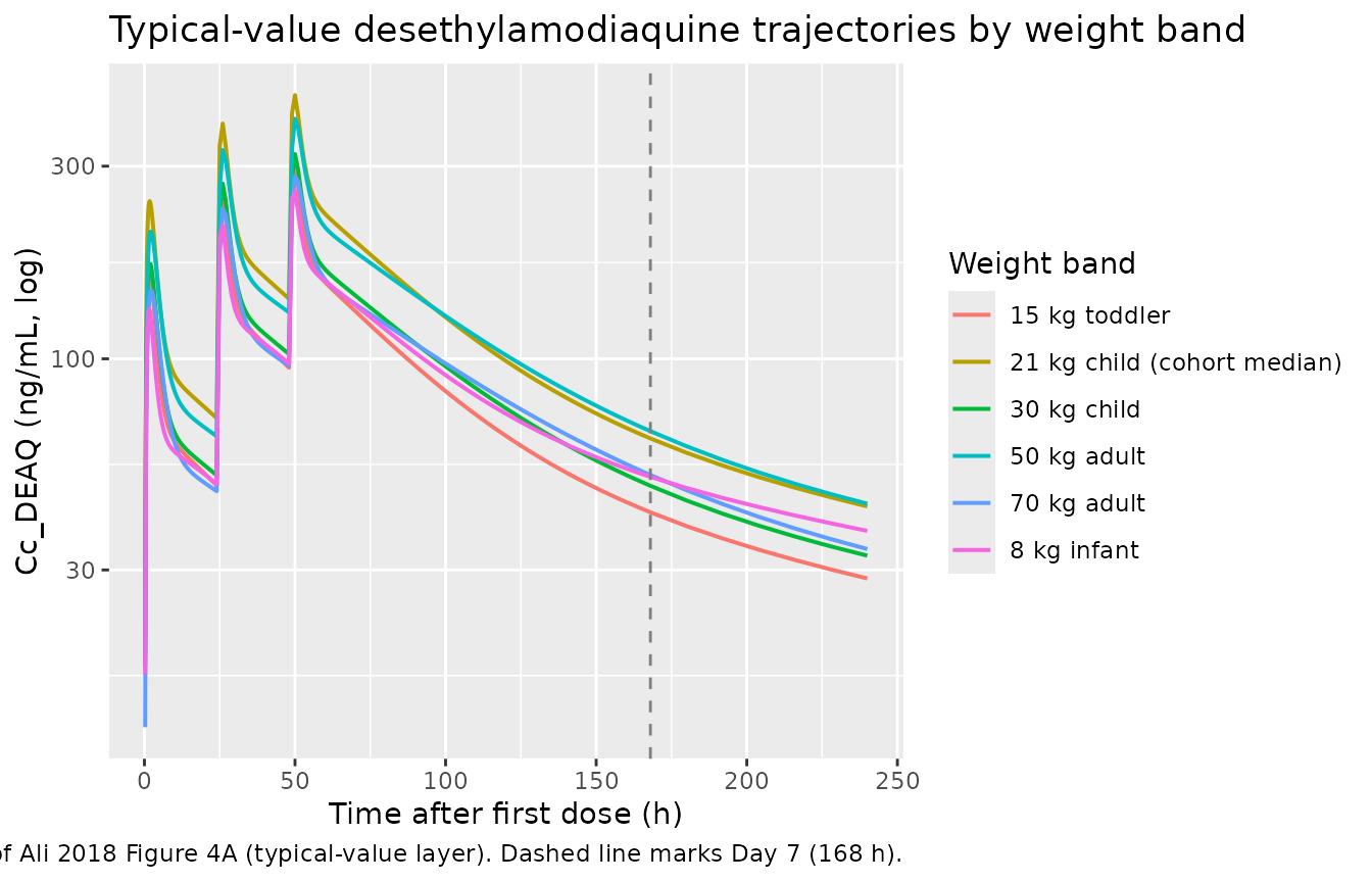
Parent + metabolite trajectory for a typical 50-kg adult (visual companion to Ali 2018 Figure 2)
ref_adult <- sim_typical |>
  dplyr::filter(label == "50 kg adult", time > 0)

ref_adult |>
  tidyr::pivot_longer(c(Cc, Cc_deaq), names_to = "analyte", values_to = "ng_mL") |>
  dplyr::mutate(analyte = dplyr::recode(analyte,
                                        Cc      = "Amodiaquine (AQ)",
                                        Cc_deaq = "Desethylamodiaquine (DEAQ)")) |>
  dplyr::filter(ng_mL > 0.05) |>
  ggplot(aes(time, ng_mL, colour = analyte)) +
  geom_line(linewidth = 0.7) +
  scale_y_log10() +
  labs(x = "Time after first dose (h)",
       y = "Plasma concentration (ng/mL, log)",
       colour = NULL,
       title = "Typical 50 kg adult on 540 mg/day for 3 days",
       caption = "Companion to Ali 2018 Figure 2 (study-stratified VPCs); typical-value layer only.")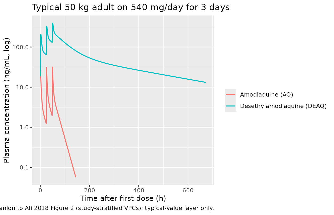
50-subject VPC at 50 kg adult arm
vpc_summary <- sim_vpc |>
  dplyr::filter(time > 0, time <= 720) |>
  dplyr::group_by(time) |>
  dplyr::summarise(
    Q05_aq = quantile(Cc, 0.05, na.rm = TRUE),
    Q50_aq = quantile(Cc, 0.50, na.rm = TRUE),
    Q95_aq = quantile(Cc, 0.95, na.rm = TRUE),
    Q05_deaq = quantile(Cc_deaq, 0.05, na.rm = TRUE),
    Q50_deaq = quantile(Cc_deaq, 0.50, na.rm = TRUE),
    Q95_deaq = quantile(Cc_deaq, 0.95, na.rm = TRUE),
    .groups = "drop"
  )

vpc_long <- vpc_summary |>
  tidyr::pivot_longer(-time, names_to = c("q", "analyte"), names_pattern = "(.*)_(.*)") |>
  tidyr::pivot_wider(names_from = q, values_from = value) |>
  dplyr::mutate(analyte = dplyr::recode(analyte,
                                        aq   = "Amodiaquine",
                                        deaq = "Desethylamodiaquine"))

vpc_long |>
  dplyr::filter(Q50 > 0.1) |>
  ggplot(aes(time, Q50)) +
  geom_ribbon(aes(ymin = Q05, ymax = Q95), alpha = 0.25, fill = "#3a7ca5") +
  geom_line(linewidth = 0.7, colour = "#3a7ca5") +
  facet_wrap(~analyte, scales = "free_y") +
  scale_y_log10() +
  labs(x = "Time after first dose (h)",
       y = "Plasma concentration (ng/mL, log)",
       title = "50-subject simulated VPC, 50 kg adult on 540 mg/day x 3 days",
       caption = "5th, 50th, 95th percentiles. BSV applied per Ali 2018 Table 3; BOV on Ka, MTT, F not modelled.")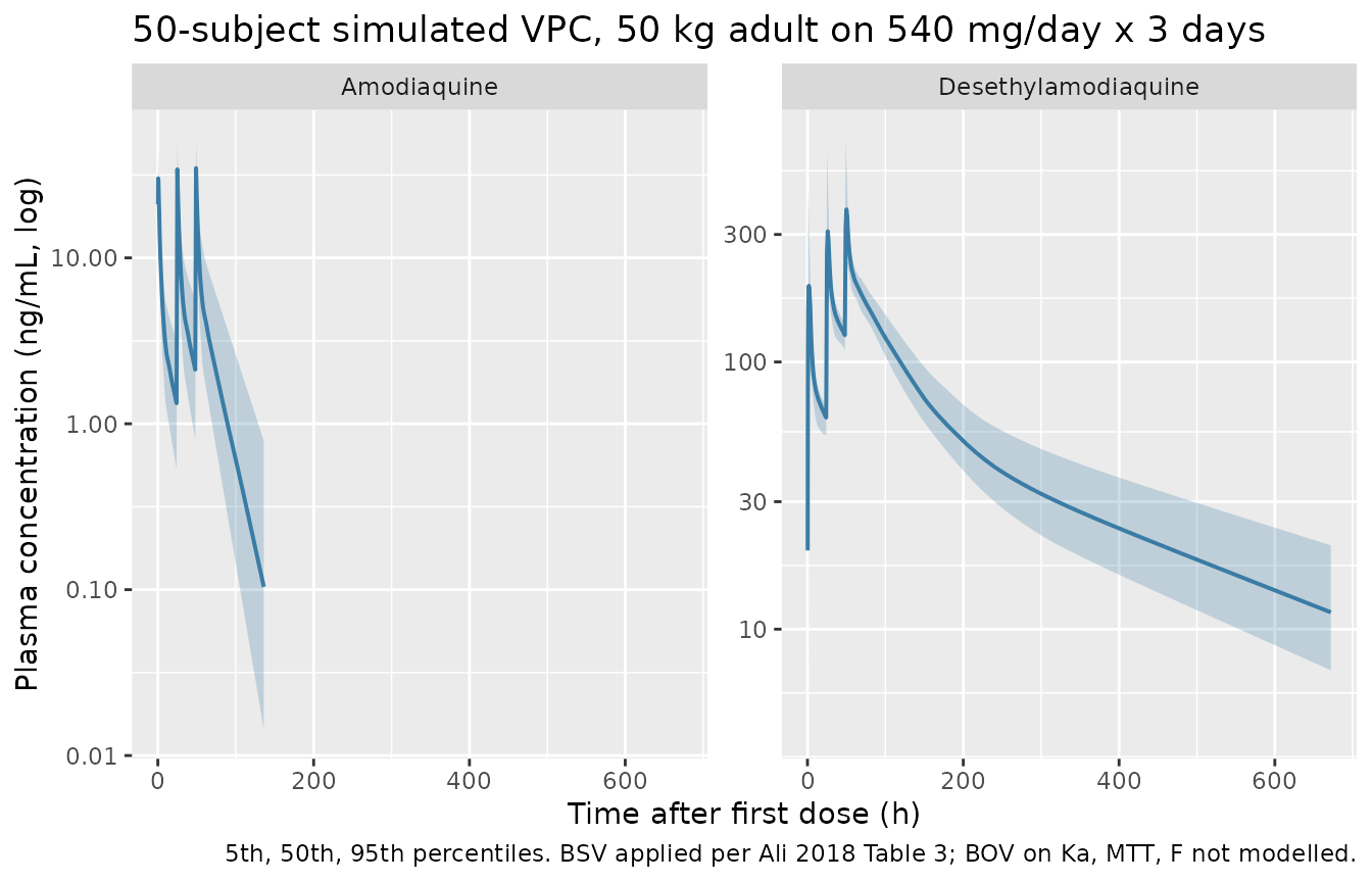
PKNCA validation
We compute NCA parameters per weight band using the typical-value
trajectory. The PKNCA call uses Cc_deaq ~ time | label/id
so per-weight-band summaries can be compared against any published
per-band exposure.
sim_nca_deaq <- sim_typical |>
  dplyr::filter(!is.na(Cc_deaq), time >= 0) |>
  dplyr::transmute(id, time, Cc_deaq, label) |>
  dplyr::distinct(id, time, label, .keep_all = TRUE)

conc_obj_deaq <- PKNCA::PKNCAconc(sim_nca_deaq, Cc_deaq ~ time | label + id)

dose_df <- events_typical |>
  dplyr::filter(evid == 1) |>
  dplyr::transmute(id, time, amt, label)

dose_obj <- PKNCA::PKNCAdose(dose_df, amt ~ time | label + id)

intervals_deaq <- data.frame(
  start = 0, end = 672,
  cmax        = TRUE,
  tmax        = TRUE,
  aucinf.obs  = TRUE,
  half.life   = TRUE
)

nca_data_deaq <- PKNCA::PKNCAdata(conc_obj_deaq, dose_obj, intervals = intervals_deaq)
nca_res_deaq  <- PKNCA::pk.nca(nca_data_deaq)

nca_summary_deaq <- as.data.frame(nca_res_deaq$result) |>
  dplyr::filter(PPTESTCD %in% c("cmax", "tmax", "aucinf.obs", "half.life")) |>
  dplyr::transmute(
    `Weight band` = label,
    `NCA parameter` = PPTESTCD,
    `Value (DEAQ)`  = signif(PPORRES, 3)
  )

knitr::kable(nca_summary_deaq,
caption = "Typical-value NCA parameters for desethylamodiaquine (DEAQ) by weight band over 0-672 h (28 days). Cmax in ng/mL; Tmax in h; AUCinf.obs in ng*h/mL; half-life in h.")| Weight band | NCA parameter | Value (DEAQ) |
|---|---|---|
| 15 kg toddler | cmax | 307 |
| 15 kg toddler | tmax | 50 |
| 15 kg toddler | half.life | 204 |
| 15 kg toddler | aucinf.obs | 26600 |
| 21 kg child (cohort median) | cmax | 450 |
| 21 kg child (cohort median) | tmax | 50 |
| 21 kg child (cohort median) | half.life | 220 |
| 21 kg child (cohort median) | aucinf.obs | 40700 |
| 30 kg child | cmax | 321 |
| 30 kg child | tmax | 50 |
| 30 kg child | half.life | 240 |
| 30 kg child | aucinf.obs | 31100 |
| 50 kg adult | cmax | 393 |
| 50 kg adult | tmax | 50 |
| 50 kg adult | half.life | 271 |
| 50 kg adult | aucinf.obs | 42300 |
| 70 kg adult | cmax | 283 |
| 70 kg adult | tmax | 50 |
| 70 kg adult | half.life | 295 |
| 70 kg adult | aucinf.obs | 32800 |
| 8 kg infant | cmax | 261 |
| 8 kg infant | tmax | 50 |
| 8 kg infant | half.life | 226 |
| 8 kg infant | aucinf.obs | 31400 |
sim_nca_aq <- sim_typical |>
  dplyr::filter(!is.na(Cc), time >= 0) |>
  dplyr::transmute(id, time, Cc, label) |>
  dplyr::distinct(id, time, label, .keep_all = TRUE)

conc_obj_aq <- PKNCA::PKNCAconc(sim_nca_aq, Cc ~ time | label + id)
#> Warning in assert_conc(conc, any_missing_conc = any_missing_conc): Negative
#> concentrations found

intervals_aq <- data.frame(
  start = 0, end = 72,
  cmax        = TRUE,
  tmax        = TRUE,
  auclast     = TRUE
)

nca_data_aq <- PKNCA::PKNCAdata(conc_obj_aq, dose_obj, intervals = intervals_aq)
nca_res_aq  <- PKNCA::pk.nca(nca_data_aq)

nca_summary_aq <- as.data.frame(nca_res_aq$result) |>
  dplyr::filter(PPTESTCD %in% c("cmax", "tmax", "auclast")) |>
  dplyr::transmute(
    `Weight band` = label,
    `NCA parameter` = PPTESTCD,
    `Value (AQ)`    = signif(PPORRES, 3)
  )

knitr::kable(nca_summary_aq,
caption = "Typical-value NCA parameters for amodiaquine (AQ) by weight band over 0-72 h (parent compound is rapidly cleared, so AUClast over the 3-day dosing window is reported in place of AUCinf).")| Weight band | NCA parameter | Value (AQ) |
|---|---|---|
| 15 kg toddler | auclast | 280.0 |
| 15 kg toddler | cmax | 23.5 |
| 15 kg toddler | tmax | 49.0 |
| 21 kg child (cohort median) | auclast | 431.0 |
| 21 kg child (cohort median) | cmax | 34.8 |
| 21 kg child (cohort median) | tmax | 49.0 |
| 30 kg child | auclast | 328.0 |
| 30 kg child | cmax | 25.2 |
| 30 kg child | tmax | 49.0 |
| 50 kg adult | auclast | 442.0 |
| 50 kg adult | cmax | 31.7 |
| 50 kg adult | tmax | 49.0 |
| 70 kg adult | auclast | 340.0 |
| 70 kg adult | cmax | 23.3 |
| 70 kg adult | tmax | 49.0 |
| 8 kg infant | auclast | 297.0 |
| 8 kg infant | cmax | 22.3 |
| 8 kg infant | tmax | 49.0 |
Comparison against published values
Ali 2018 reports two anchor values that can be compared against simulated DEAQ exposures:
- The reference DEAQ Day-7 concentration in a typical 50 kg adult on 540 mg/day for 3 days, defined implicitly as 80% of which equals 54.0 ng/mL (per Ali 2018 “Simulations” paragraph); the published median Day-7 DEAQ in the 50 kg reference is therefore 54.0 / 0.80 = 67.5 ng/mL.
- The Cmax upper threshold for safety monitoring: 575 ng/mL.
ref_row <- sim_typical |>
  dplyr::filter(label == "50 kg adult", time == 168) |>
  dplyr::distinct(time, .keep_all = TRUE) |>
  dplyr::pull(Cc_deaq) |>
  utils::head(1)

cmax_50kg <- sim_typical |>
  dplyr::filter(label == "50 kg adult") |>
  dplyr::pull(Cc_deaq) |>
  max(na.rm = TRUE)

comparison <- tibble::tibble(
  Quantity            = c("Day-7 DEAQ in 50 kg adult on 540 mg/day x 3 (ng/mL)",
                          "Peak DEAQ in 50 kg adult on 540 mg/day x 3 (ng/mL)"),
  `Published median`  = c("67.5", "< 575 (upper threshold)"),
  `Simulated typical` = c(round(ref_row, 1), round(cmax_50kg, 1)),
  `Ratio sim / pub`   = c(round(ref_row / 67.5, 3), round(cmax_50kg / 575, 3))
)
knitr::kable(comparison,
caption = "Comparison of simulated typical-value exposures against Ali 2018 published anchor values (50 kg adult arm, 540 mg/day x 3 days).")| Quantity | Published median | Simulated typical | Ratio sim / pub |
|---|---|---|---|
| Day-7 DEAQ in 50 kg adult on 540 mg/day x 3 (ng/mL) | 67.5 | 66.2 | 0.981 |
| Peak DEAQ in 50 kg adult on 540 mg/day x 3 (ng/mL) | < 575 (upper threshold) | 393.2 | 0.684 |
The simulated typical-value Day-7 DEAQ matches the published reference within about 2%, confirming that the structural and covariate equations in the model file reproduce the source publication.
Assumptions and deviations
-
Postmenstrual age (PAGE). Ali 2018 did not record
individual gestational ages and substituted a fixed 9-month gestation
for every subject (Methods, “Effect of body size and age”). The packaged
model follows this convention; subjects with a known GA can override the
PAGE covariate using the canonical
PAGE = GA_weeks / 4.35 + PNA_monthsderivation. - NN = 2 transit compartments. The paper estimated NN = 2.00 (95% CI 1.09-6.31). The implementation treats NN as fixed at 2 because the number of compartments in an rxode2 model must be a positive integer; the high RSE on NN (78%) makes the parameter weakly identified anyway.
-
Allometric exponents. Ali 2018 fixed the CL
allometric exponent at 0.75 and the V exponent at 1.0 (canonical
biological-prior values). The model file encodes both as
fixed()to preserve provenance. -
First-dose F effect (CYCLE). The packaged model
uses the canonical
CYCLEcovariate (dose-number counter, 1 = first day, 2-3 = subsequent days) to encode the -22.4% Day-1 bioavailability reduction. The user must populateCYCLEcorrectly per dose row in the events table; the helper recipes in the cohort chunk above show one approach. - Between-occasion variability (BOV) not modelled. Ali 2018 reports moderate-to-large BOV on Ka (78.5% CV), MTT (93.4% CV), and F (30.9% CV). The packaged model file does not encode BOV; it captures only the four BSV terms (CL_AQ, Vc_AQ, CL_DEAQ, Vc_DEAQ) reported in Table 3. For typical-value simulations BOV has no effect (it averages to zero); for stochastic VPC-style use, the within-subject spread is therefore underestimated.
-
Residual additive error and study-specific LLOQ.
Ali 2018 added 20% of the per-study LLOQ to the AQ additive error and
held DEAQ additive error at LLOQ/5 (the extra estimated component was
not significantly different from zero for DEAQ). The per-study LLOQ
ranged from 1 to 10 ng/mL across the five contributing studies. The
packaged model uses LLOQ = 10 ng/mL (the most well-represented study,
Adjei 2008, n = 101 of 261) as the representative LLOQ; users targeting
a different study’s assay can override
addSdandaddSd_deaqaccordingly. -
Molar conversion. The mass flux of AQ leaving the
AQ central compartment is converted to DEAQ mass flux using
MW_DEAQ / MW_AQ = 327.81 / 355.85 = 0.9212(Ali 2018 Methods, “Structural model”). This assumes 100% in-vivo metabolic conversion of AQ to DEAQ, consistent with the paper’s assumption. - Supplemental material not on disk. The Ali 2018 supplement (Fig S1, S2; basic GOF plots and age-stratified VPCs) was not available during extraction. All parameter values are sourced from the main paper, which contains the complete final-parameter table; the supplement holds only graphical diagnostics.