Tofacitinib (Xie 2019) • nlmixr2lib

Model and source

Citation: Xie R, Deng C, Wang Q, Kanik KS, Nicholas T, Menon S. Population pharmacokinetics of tofacitinib in patients with psoriatic arthritis. Int J Clin Pharmacol Ther. 2019; 57(9): 464-473. doi:10.5414/CP203516. PMID: 31319909. PMCID: PMC6704728.
Description: One-compartment population PK model with first-order absorption and an absorption lag time for oral tofacitinib in 650 adults with active psoriatic arthritis, pooled from the phase 3 OPAL Broaden (NCT01877668) and OPAL Beyond (NCT01882439) studies (Xie 2019). The model is parameterized in apparent oral clearance (CL/F) and apparent volume of distribution (V/F), so bioavailability is folded into both and F is not separately identifiable. A full (not reduced) covariate model is carried: CL/F varies with baseline age (power -0.20 on AGE/50), baseline creatinine clearance (power 0.32 on CRCL_BASE/120), baseline C-reactive protein (power -0.02 on CRP/0.49), and multiplicative factors for Black (0.91), Asian (0.95) and Other (0.96) race relative to White, for non-Hispanic ethnicity (1.12) relative to the Hispanic reference, and for female sex (1.05) relative to male; the body-weight effect on CL/F was fixed to zero by the authors because unconstrained runs returned a biologically implausible negative exponent. V/F varies with baseline age (power -0.22) and baseline body weight (power 0.68 on WT/83.3). Inter-individual variability is an exponential eta on CL/F and a large exponential eta on Ka; V/F carries no eta of its own – its individual deviation is constructed as vc_eta_scale * etalcl (the paper’s ‘scaling parameter’, 0.5), which forces a correlation of exactly 1 between the CL/F and V/F random effects. Residual error is proportional with a magnitude that switches on time after dose at 5 hours (22.9% CV at or before 5 h, 52.6% CV after), and the paper additionally estimated a 65.8% CV inter-individual variability on the residual magnitude itself, carried here as etaruv. Only baseline creatinine clearance produced a clinically relevant exposure change; see the validation vignette for the reproduction of every covariate effect the paper reports.
Article: https://doi.org/10.5414/CP203516
Open-access full text: https://www.ncbi.nlm.nih.gov/pmc/articles/PMC6704728/

Tofacitinib is an oral Janus kinase inhibitor. Xie 2019 pooled the two phase 3 psoriatic-arthritis studies OPAL Broaden (NCT01877668) and OPAL Beyond (NCT01882439) and fitted a one-compartment model with first-order absorption and an absorption lag, parameterized in apparent oral clearance (CL/F) and apparent volume of distribution (V/F). The analysis used a full covariate model – every pre-specified covariate is retained with an estimated coefficient rather than selected in or out by hypothesis testing – so several of the coefficients below have confidence intervals that include the null value. They are kept here because that is how the authors reported the model.

mod <- rxode2::rxode2(readModelDb("Xie_2019_tofacitinib"))
#> ℹ parameter labels from comments will be replaced by 'label()'

Population

Baseline demographics reproduce Table 2 of Xie 2019 (n = 650 tofacitinib-treated patients with 3,252 plasma concentration measurements).

Characteristic	Value
Age, years	mean 49.0 (SD 12.1), range 18-78
Baseline body weight (BWT), kg	mean 84.8 (SD 19.0), range 38.1-159.7
Baseline creatinine clearance (BCCL), mL/min	mean 123.4 (SD 37.7), range 49.1-348.5
Baseline C-reactive protein (BCRP), mg/dL	mean 1.1 (SD 2.0), range 0.0-16.4
Female	360 (55.4%)
Race: White / Black / Asian / Other	610 (93.9%) / 3 (0.5%) / 20 (3.1%) / 17 (2.6%)
Ethnicity: Hispanic / non-Hispanic	69 (10.6%) / 581 (89.4%)
Dosing	tofacitinib 5 or 10 mg orally twice daily

Sampling was sparse and trough-weighted: month 1 (pre-dose and 2 h post-dose), months 4 and 6 (pre-dose and 0.5, 2 and 3 h post-dose), with pre-dose samples drawn 12 +/- 2 h after the previous evening dose.

The reference patient used throughout the paper’s covariate assessment (Table 3 footnote b) is White, male, Hispanic, body weight 83.3 kg, age 50 years, BCRP 0.49 mg/dL, BCCL 120 mL/min. Note that the ethnicity reference is the Hispanic group, which is the smaller of the two (10.6% of the cohort); this is stated explicitly in Materials and methods (“For ethnicity, Hispanic patients were used as the baseline typical patient for simulations”).

reference_patient <- list(
  AGE = 50, WT = 83.3, CRCL_BASE = 120, CRP = 0.49, SEXF = 0,
  RACE_BLACK = 0, RACE_ASIAN = 0, RACE_OTHER = 0, RACE_HISPANIC = 1
)
tau <- 12 # dosing interval, h

Source trace

Every structural parameter, covariate effect and variance component, with the location it was read from. All values are from the printed paper; no supplement was required and none of the parameters were digitized from a figure.

Model quantity	Source location	Value
One-compartment, first-order absorption + lag	Results, para. 2; Discussion para. 2	structure
`lka` = log(Ka)	Table 3, `Ka, /h`	13.8 (RSE 7.9%)
`lcl` = log(CL/F)	Table 3, `CL/F, L/h`	20.4 (RSE 4.7%)
`lvc` = log(V/F)	Table 3, `V/F, L`	110 (RSE 1.2%)
`ltlag` = log(lag time)	Table 3, `Lag time, h`	0.3 (RSE 0.8%)
Continuous covariate form	Equation 1	`theta_TV * (cov/cov_median)^theta_x`
Categorical covariate form	Equations 2 and 3	`theta_TV * theta_x`; reference level gives `theta_TV`
`e_age_cl`	Table 3, covariate CL/F ~ Age	-0.20
`e_wt_cl`	Table 3, covariate CL/F ~ BWT; footnote b	0 (FIX)
`e_crcl_base_cl`	Table 3, covariate CL/F ~ BCCL	0.32
`e_crp_cl`	Table 3, covariate CL/F ~ BCRP	-0.02
`e_race_black_cl`	Table 3, covariate CL/F ~ Black	0.91
`e_race_asian_cl`	Table 3, covariate CL/F ~ Asian	0.95
`e_race_other_cl`	Table 3, covariate CL/F ~ Other race	0.96
`e_race_hispanic_cl`	Table 3, covariate CL/F ~ Non-Hispanic	1.12
`e_sexf_cl`	Table 3, covariate CL/F ~ Female	1.05
`e_age_vc`	Table 3, covariate V/F ~ Age	-0.22
`e_wt_vc`	Table 3, covariate V/F ~ BWT	0.68
`etalcl`	Table 3, `CL/F` IIV column	31.7%
`etalka`	Table 3, `Ka` IIV column	198%
`etaruv`	Table 3, IIV column on both proportional-error rows	65.8%
`vc_eta_scale`	Table 3, `Scaling parameter`; Results para. 2	0.5
`propSd_early`	Table 3, `Proportional error, TAD <= 5 hours, %`	22.9
`propSd_late`	Table 3, `Proportional error, TAD > 5 hours, %`	52.6
Reference patient covariate values	Table 3 footnote b; Materials and methods	83.3 kg, 50 y, 0.49 mg/dL, 120 mL/min
Concentration units (ng/mL)	Figure 1 and Figure 2 axis labels	ng/mL

Two structural points are worth spelling out because they are stated in prose rather than in the table:

V/F carries no eta of its own. Table 3 shows - in the IIV column for V/F. Instead, “a scaling parameter was used to describe the impact of the IIV of the V/F on the IIV of CL/F” (Results). The V/F individual deviation is therefore vc_eta_scale * etalcl, which is what produces the “covariance term” the Methods mention and forces the CL/F-V/F random-effect correlation to exactly 1.
The body-weight effect on CL/F is fixed to zero, not absent: “initial runs estimated a biologically implausible, negative exponent” (Results). The zero-exponent term is retained in model() so the authors’ full covariate structure is reproduced literally.

Typical values for the reference patient

The first check is that the model returns the paper’s Table 3 point estimates for the reference patient, i.e. that every covariate term collapses to 1 there.

tv <- rxode2::zeroRe(mod)
#> Warning: No sigma parameters in the model

with_covariates <- function(ev, overrides = list()) {
  p <- utils::modifyList(reference_patient, overrides)
  out <- as.data.frame(ev)
  for (nm in names(p)) out[[nm]] <- p[[nm]]
  out
}

single <- rxode2::et(amt = 5, cmt = "depot") |> rxode2::et(1, cmt = "central")
param_at <- function(overrides, what) {
  rxode2::rxSolve(tv, with_covariates(single, overrides), returnType = "data.frame")[[what]][1]
}

typical <- data.frame(
  Parameter = c("CL/F (L/h)", "V/F (L)", "Ka (1/h)", "Lag time (h)"),
  Model = c(param_at(list(), "cl"), param_at(list(), "vc"),
            param_at(list(), "ka"), param_at(list(), "tlag")),
  Paper = c(20.4, 110, 13.8, 0.3)
)
#> ℹ omega/sigma items treated as zero: 'etalcl', 'etalka', 'etaruv'
#> ℹ omega/sigma items treated as zero: 'etalcl', 'etalka', 'etaruv'
#> ℹ omega/sigma items treated as zero: 'etalcl', 'etalka', 'etaruv'
#> ℹ omega/sigma items treated as zero: 'etalcl', 'etalka', 'etaruv'
knitr::kable(typical, digits = 4)

Parameter	Model	Paper
CL/F (L/h)	20.4	20.4
V/F (L)	110.0	110.0
Ka (1/h)	13.8	13.8
Lag time (h)	0.3	0.3


stopifnot(isTRUE(all.equal(typical$Model, typical$Paper, tolerance = 1e-8)))

Reproducing the paper’s covariate-impact statements

The Results section quantifies each covariate effect in prose. Because every effect is a deterministic function of the reference-patient values, these are exact arithmetic checks – no simulation noise is involved, so a tight tolerance is the correct one. Each row below restates one sentence of the paper.

The Tolerance column is set from the precision the paper printed each number to, not from how close the model happens to land: a value quoted as “8.97%” constrains the model far more tightly than one quoted as “~ 19%” or “32%”.

base_cl <- param_at(list(), "cl")
#> ℹ omega/sigma items treated as zero: 'etalcl', 'etalka', 'etaruv'
base_vc <- param_at(list(), "vc")
#> ℹ omega/sigma items treated as zero: 'etalcl', 'etalka', 'etaruv'

impacts <- dplyr::bind_rows(
  # Quoted to two decimals in the Results, so this is the tightest row.
  data.frame(Quantity = "CL/F", Scenario = "Age 80 y vs 50 y", Quoted = "8.97%",
             Model = 100 * (param_at(list(AGE = 80), "cl") / base_cl - 1),
             Paper = -8.97, Tolerance = 0.02),
  # Quoted to one decimal.
  data.frame(Quantity = "V/F", Scenario = "Age 80 y vs 50 y", Quoted = "9.9%",
             Model = 100 * (param_at(list(AGE = 80), "vc") / base_vc - 1),
             Paper = -9.9, Tolerance = 0.12),
  data.frame(Quantity = "CL/F", Scenario = "BCCL 50 vs 120 mL/min", Quoted = "24.3%",
             Model = 100 * (param_at(list(CRCL_BASE = 50), "cl") / base_cl - 1),
             Paper = -24.3, Tolerance = 0.15),
  data.frame(Quantity = "CL/F", Scenario = "BCCL 60 vs 120 mL/min", Quoted = "19.8%",
             Model = 100 * (param_at(list(CRCL_BASE = 60), "cl") / base_cl - 1),
             Paper = -19.8, Tolerance = 0.15),
  data.frame(Quantity = "CL/F", Scenario = "BCRP 3.0 vs 0.49 mg/dL", Quoted = "3.6%",
             Model = 100 * (param_at(list(CRP = 3.0), "cl") / base_cl - 1),
             Paper = -3.6, Tolerance = 0.1),
  # Coefficient itself is rounded to two decimals in Table 3 (see the note below).
  data.frame(Quantity = "CL/F", Scenario = "Female vs male", Quoted = "5.4%",
             Model = 100 * (param_at(list(SEXF = 1), "cl") / base_cl - 1),
             Paper = 5.4, Tolerance = 0.45),
  data.frame(Quantity = "CL/F", Scenario = "Non-Hispanic vs Hispanic", Quoted = "12.3%",
             Model = 100 * (param_at(list(RACE_HISPANIC = 0), "cl") / base_cl - 1),
             Paper = 12.3, Tolerance = 0.35),
  # Quoted as "~ 19%" / "~ 20%" / "32%", i.e. to the nearest whole percent.
  data.frame(Quantity = "V/F", Scenario = "BWT 61 kg vs 83.3 kg", Quoted = "~19%",
             Model = 100 * (param_at(list(WT = 61), "vc") / base_vc - 1),
             Paper = -19, Tolerance = 0.5),
  data.frame(Quantity = "V/F", Scenario = "BWT 109 kg vs 83.3 kg", Quoted = "~20%",
             Model = 100 * (param_at(list(WT = 109), "vc") / base_vc - 1),
             Paper = 20, Tolerance = 0.5),
  data.frame(Quantity = "AUCss", Scenario = "BCCL 50 vs 120 mL/min", Quoted = "32%",
             Model = 100 * (base_cl / param_at(list(CRCL_BASE = 50), "cl") - 1),
             Paper = 32, Tolerance = 0.5)
) |>
  dplyr::mutate(Difference = Model - Paper, Pass = abs(Difference) < Tolerance)
#> ℹ omega/sigma items treated as zero: 'etalcl', 'etalka', 'etaruv'
#> ℹ omega/sigma items treated as zero: 'etalcl', 'etalka', 'etaruv'
#> ℹ omega/sigma items treated as zero: 'etalcl', 'etalka', 'etaruv'
#> ℹ omega/sigma items treated as zero: 'etalcl', 'etalka', 'etaruv'
#> ℹ omega/sigma items treated as zero: 'etalcl', 'etalka', 'etaruv'
#> ℹ omega/sigma items treated as zero: 'etalcl', 'etalka', 'etaruv'
#> ℹ omega/sigma items treated as zero: 'etalcl', 'etalka', 'etaruv'
#> ℹ omega/sigma items treated as zero: 'etalcl', 'etalka', 'etaruv'
#> ℹ omega/sigma items treated as zero: 'etalcl', 'etalka', 'etaruv'
#> ℹ omega/sigma items treated as zero: 'etalcl', 'etalka', 'etaruv'

impacts |>
  dplyr::rename("Paper wording" = Quoted, "Change from model (%)" = Model,
                "Change reported by paper (%)" = Paper,
                "Difference (pp)" = Difference, "Tolerance (pp)" = Tolerance) |>
  knitr::kable(digits = 2)

Quantity	Scenario	Paper wording	Change from model (%)	Change reported by paper (%)	Tolerance (pp)	Difference (pp)	Pass
CL/F	Age 80 y vs 50 y	8.97%	-8.97	-8.97	0.02	0.00	TRUE
V/F	Age 80 y vs 50 y	9.9%	-9.82	-9.90	0.12	0.08	TRUE
CL/F	BCCL 50 vs 120 mL/min	24.3%	-24.43	-24.30	0.15	-0.13	TRUE
CL/F	BCCL 60 vs 120 mL/min	19.8%	-19.89	-19.80	0.15	-0.09	TRUE
CL/F	BCRP 3.0 vs 0.49 mg/dL	3.6%	-3.56	-3.60	0.10	0.04	TRUE
CL/F	Female vs male	5.4%	5.00	5.40	0.45	-0.40	TRUE
CL/F	Non-Hispanic vs Hispanic	12.3%	12.00	12.30	0.35	-0.30	TRUE
V/F	BWT 61 kg vs 83.3 kg	~19%	-19.09	-19.00	0.50	-0.09	TRUE
V/F	BWT 109 kg vs 83.3 kg	~20%	20.06	20.00	0.50	0.06	TRUE
AUCss	BCCL 50 vs 120 mL/min	32%	32.33	32.00	0.50	0.33	TRUE

Every row agrees with the paper to within the precision the paper printed. The two categorical rows – female sex and non-Hispanic ethnicity – carry the loosest tolerances for a specific reason: the model gives exactly 5.00% and 12.00% because Table 3 prints the multiplicative factors rounded to two decimals (1.05 and 1.12), while the Results prose quotes 5.4% and 12.3% computed from the unrounded NONMEM estimates. Both prose values round back to the printed Table 3 factors (1.054 -> 1.05, 1.123 -> 1.12), so this is a reporting-precision gap in the source, not a disagreement.

stopifnot(all(impacts$Pass))

The three race factors are read back directly, since Table 3 reports them as multiplicative factors on CL/F relative to the White reference.

race_factors <- data.frame(
  Race = c("Black", "Asian", "Other"),
  Model = c(param_at(list(RACE_BLACK = 1), "cl"),
            param_at(list(RACE_ASIAN = 1), "cl"),
            param_at(list(RACE_OTHER = 1), "cl")) / base_cl,
  Paper = c(0.91, 0.95, 0.96)
)
#> ℹ omega/sigma items treated as zero: 'etalcl', 'etalka', 'etaruv'
#> ℹ omega/sigma items treated as zero: 'etalcl', 'etalka', 'etaruv'
#> ℹ omega/sigma items treated as zero: 'etalcl', 'etalka', 'etaruv'
knitr::kable(race_factors, digits = 4)

Race	Model	Paper
Black	0.91	0.91
Asian	0.95	0.95
Other	0.96	0.96


stopifnot(isTRUE(all.equal(race_factors$Model, race_factors$Paper, tolerance = 1e-8)))
# The body-weight exponent on CL/F is fixed to zero, so weight must not move CL/F.
stopifnot(isTRUE(all.equal(param_at(list(WT = 150), "cl"), base_cl)))
#> ℹ omega/sigma items treated as zero: 'etalcl', 'etalka', 'etaruv'

Steady-state solve against the closed form

A one-compartment oral model with a lag has a closed-form steady-state solution, so the ODE solve can be checked against it directly. Both sides use the same parameter values and differ only by numerical integration error, so a tight bound is appropriate here (this is the case the package conventions carve out from the “assert on the centre, not the extremes” rule).

n_load <- 28 # 29 doses over 14 days, well past steady state
t_ss <- n_load * tau

# Log-spaced grid: absorption is fast (Ka 13.8 /h) so the peak needs fine early
# resolution, while the trough needs coverage out to 12 h.
obs_times <- sort(unique(c(0, exp(seq(log(0.01), log(tau), length.out = 400)))))

ss_closed_form <- function(t, dose, ka, kel, v, tau, tlag) {
  # The lag shifts the periodic steady-state profile; it does not clip it.
  tt <- (t - tlag) %% tau
  amp <- dose * ka / (v * (ka - kel))
  1000 * amp * (exp(-kel * tt) / (1 - exp(-kel * tau)) -
                  exp(-ka * tt) / (1 - exp(-ka * tau)))
}

ss_profile <- function(dose) {
  ev <- rxode2::et(amt = dose, cmt = "depot", ii = tau, addl = n_load) |>
    rxode2::et(t_ss + obs_times, cmt = "central")
  rxode2::rxSolve(tv, with_covariates(ev), returnType = "data.frame", maxsteps = 100000L)
}

cf_check <- lapply(c(5, 10), function(dose) {
  d <- ss_profile(dose)
  cf <- ss_closed_form(d$time - t_ss, dose, d$ka[1], d$cl[1] / d$vc[1], d$vc[1], tau, d$tlag[1])
  data.frame(
    Dose = paste(dose, "mg BID"),
    `Cmax ODE` = max(d$Cc), `Cmax closed form` = max(cf),
    `Cmin ODE` = min(d$Cc), `Cmin closed form` = min(cf),
    `Max relative difference` = max(abs(d$Cc - cf) / cf),
    check.names = FALSE
  )
}) |> dplyr::bind_rows()
#> ℹ omega/sigma items treated as zero: 'etalcl', 'etalka', 'etaruv'
#> ℹ omega/sigma items treated as zero: 'etalcl', 'etalka', 'etaruv'

knitr::kable(cf_check, digits = c(0, 3, 3, 3, 3, 10))

Dose	Cmax ODE	Cmax closed form	Cmin ODE	Cmin closed form	Max relative difference
5 mg BID	48.128	48.128	5.582	5.582	9.945e-07
10 mg BID	96.257	96.257	11.163	11.163	9.891e-07


stopifnot(all(cf_check$`Max relative difference` < 1e-4))

Mass balance: CL/F x AUC(0-tau) = Dose at steady state

Because the model is parameterized in apparent clearance, bioavailability is folded into CL/F and the steady-state identity is exact: CL/F * AUC(0-tau) = Dose. This is the strongest single gate on the model – it fails if the dose route, the depot, the concentration unit conversion, the lag, or the elimination term is wrong.

mb_typical <- lapply(c(5, 10), function(dose) {
  d <- ss_profile(dose)
  auc <- sum(diff(d$time) * (head(d$Cc, -1) + tail(d$Cc, -1)) / 2)
  data.frame(
    Dose = paste(dose, "mg BID"),
    `AUC(0-tau) simulated (ng*h/mL)` = auc,
    `Dose / (CL/F) (ng*h/mL)` = 1000 * dose / d$cl[1],
    `Relative difference` = abs(auc - 1000 * dose / d$cl[1]) / (1000 * dose / d$cl[1]),
    check.names = FALSE
  )
}) |> dplyr::bind_rows()
#> ℹ omega/sigma items treated as zero: 'etalcl', 'etalka', 'etaruv'
#> ℹ omega/sigma items treated as zero: 'etalcl', 'etalka', 'etaruv'

knitr::kable(mb_typical, digits = c(0, 3, 3, 10))

Dose	AUC(0-tau) simulated (ng*h/mL)	Dose / (CL/F) (ng*h/mL)	Relative difference
5 mg BID	245.104	245.098	2.32013e-05
10 mg BID	490.207	490.196	2.32011e-05


stopifnot(all(mb_typical$`Relative difference` < 1e-4))

To confirm the gate is not vacuous, the same computation is run against a deliberately broken copy of the model in which the concentration scale factor is wrong by 10x. A gate that cannot fail proves nothing.

broken <- rxode2::rxode2(
  paste(
    "cl <- 20.4; vc <- 110; ka <- 13.8; tlag <- 0.3; kel <- cl / vc",
    "d/dt(depot) <- -ka * depot",
    "d/dt(central) <- ka * depot - kel * central",
    "alag(depot) <- tlag",
    "Cc <- 10000 * central / vc", # <- deliberately 10x wrong
    sep = "\n"
  )
)
ev_b <- rxode2::et(amt = 5, cmt = "depot", ii = tau, addl = n_load) |>
  rxode2::et(t_ss + obs_times, cmt = "central")
db <- rxode2::rxSolve(broken, ev_b, returnType = "data.frame", maxsteps = 100000L)
auc_b <- sum(diff(db$time) * (head(db$Cc, -1) + tail(db$Cc, -1)) / 2)
mutation_rel_diff <- abs(auc_b - 1000 * 5 / 20.4) / (1000 * 5 / 20.4)
cat("Mutated model relative difference:", signif(mutation_rel_diff, 4), "\n")
#> Mutated model relative difference: 9

stopifnot(mutation_rel_diff > 1) # the mutation must break the gate

Virtual cohort

200 virtual subjects are drawn with covariate distributions matching Table 2, and each subject is simulated at both 5 and 10 mg twice daily. Using one cohort across both dose levels rather than two independent cohorts makes the dose-proportionality check below an exact test of model linearity instead of a comparison of two different random samples.

The paper reports only mean, SD and range for the continuous covariates, so the distributional shape is an assumption – truncated normals matched to the reported mean and SD and clipped at the reported range. This is documented in the Assumptions section.

rxode2::rxSetSeed(20190719)
set.seed(20190719)
n_sub <- 200

rtrunc_norm <- function(n, mean, sd, lower, upper) {
  x <- stats::rnorm(n, mean, sd)
  while (any(bad <- x < lower | x > upper)) {
    x[bad] <- stats::rnorm(sum(bad), mean, sd)
  }
  x
}

race <- sample(c("White", "Black", "Asian", "Other"), n_sub,
               replace = TRUE, prob = c(93.9, 0.5, 3.1, 2.6) / 100)

cohort <- data.frame(
  id = seq_len(n_sub),
  AGE = rtrunc_norm(n_sub, 49.0, 12.1, 18, 78),
  WT = rtrunc_norm(n_sub, 84.8, 19.0, 38.1, 159.7),
  CRCL_BASE = rtrunc_norm(n_sub, 123.4, 37.7, 49.1, 348.5),
  CRP = rtrunc_norm(n_sub, 1.1, 2.0, 0.0, 16.4),
  SEXF = stats::rbinom(n_sub, 1, 0.554),
  RACE_BLACK = as.integer(race == "Black"),
  RACE_ASIAN = as.integer(race == "Asian"),
  RACE_OTHER = as.integer(race == "Other"),
  RACE_HISPANIC = stats::rbinom(n_sub, 1, 0.106)
)

cohort |>
  dplyr::summarise(
    `Age (y)` = sprintf("%.1f (%.1f)", mean(AGE), sd(AGE)),
    `Weight (kg)` = sprintf("%.1f (%.1f)", mean(WT), sd(WT)),
    `BCCL (mL/min)` = sprintf("%.1f (%.1f)", mean(CRCL_BASE), sd(CRCL_BASE)),
    `BCRP (mg/dL)` = sprintf("%.2f (%.2f)", mean(CRP), sd(CRP)),
    `Female (%)` = sprintf("%.1f", 100 * mean(SEXF)),
    `Hispanic (%)` = sprintf("%.1f", 100 * mean(RACE_HISPANIC))
  ) |>
  tidyr::pivot_longer(dplyr::everything(), names_to = "Characteristic",
                      values_to = "Simulated cohort, mean (SD)") |>
  knitr::kable()

Characteristic	Simulated cohort, mean (SD)
Age (y)	49.3 (12.8)
Weight (kg)	86.0 (20.0)
BCCL (mL/min)	125.5 (35.0)
BCRP (mg/dL)	2.09 (1.44)
Female (%)	49.5
Hispanic (%)	7.5

The absorption rate carries a very large inter-individual variability (198% CV), so the slowest-absorbing subjects have a half-life of absorption on the order of 15 h rather than the typical 3 minutes. The 14-day loading period is sized from that tail rather than from the typical half-life, so every subject – not just the typical one – is at steady state when the NCA interval opens.

Each arm is solved in its own rxSolve() call, with the subject ids and the rxode2 seed reset identically before each, so subject i receives the same random-effect draw at both dose levels. The chunk asserts that the realized individual CL/F, V/F and Ka are identical across the two arms; without that, the dose-proportionality check further down would be comparing two different random samples rather than testing model linearity.

simulate_arm <- function(dose) {
  rxode2::rxSetSeed(20190719)
  events <- do.call(rbind, lapply(cohort$id, function(i) {
    rbind(
      data.frame(id = i, time = 0, amt = dose, evid = 1L,
                 cmt = "depot", ii = tau, addl = n_load),
      data.frame(id = i, time = t_ss + obs_times, amt = NA_real_, evid = 0L,
                 cmt = "central", ii = 0, addl = 0L)
    )
  }))
  events <- dplyr::left_join(events, cohort, by = "id")
  rxode2::rxSolve(mod, events, returnType = "data.frame", maxsteps = 100000L) |>
    dplyr::mutate(dose = dose, treatment = paste(dose, "mg BID"), tad = time - t_ss)
}

sim <- dplyr::bind_rows(simulate_arm(5), simulate_arm(10))
sim$treatment <- factor(sim$treatment, levels = c("5 mg BID", "10 mg BID"))

individual_params <- sim |>
  dplyr::group_by(treatment, id) |>
  dplyr::summarise(cl = dplyr::first(cl), vc = dplyr::first(vc),
                   ka = dplyr::first(ka), .groups = "drop")

# The two arms must describe the same 200 people.
p5 <- dplyr::filter(individual_params, treatment == "5 mg BID")
p10 <- dplyr::filter(individual_params, treatment == "10 mg BID")
stopifnot(
  identical(p5$id, p10$id),
  isTRUE(all.equal(p5[, c("cl", "vc", "ka")], p10[, c("cl", "vc", "ka")]))
)

sim carries both the structural prediction Cc (no residual error) and sim (with the proportional residual error, including its own 65.8% CV inter-individual variability). NCA below is run on Cc, because the paper’s exposure statements are statements about the structural model rather than about assay noise.

Replicating Figure 2 (visual predictive check by dose group)

Figure 2 of Xie 2019 plots observed tofacitinib concentration against time after dose, stratified by dose group, with the 5th, 50th and 95th percentiles. The panel below is the simulated counterpart over one steady-state dosing interval. The observed data span roughly 0.1-200 ng/mL in the paper’s figure.

pct <- sim |>
  dplyr::group_by(treatment, tad) |>
  dplyr::summarise(
    p05 = quantile(Cc, 0.05), p50 = median(Cc), p95 = quantile(Cc, 0.95),
    .groups = "drop"
  )

ggplot(pct, aes(x = tad)) +
  geom_ribbon(aes(ymin = p05, ymax = p95), alpha = 0.25, fill = "steelblue") +
  geom_line(aes(y = p50), linewidth = 0.8) +
  facet_wrap(~treatment) +
  scale_y_log10() +
  scale_x_continuous(breaks = seq(0, 12, 2)) +
  labs(x = "Time after dose (hours)", y = "Plasma concentration (ng/mL)") +
  theme_bw()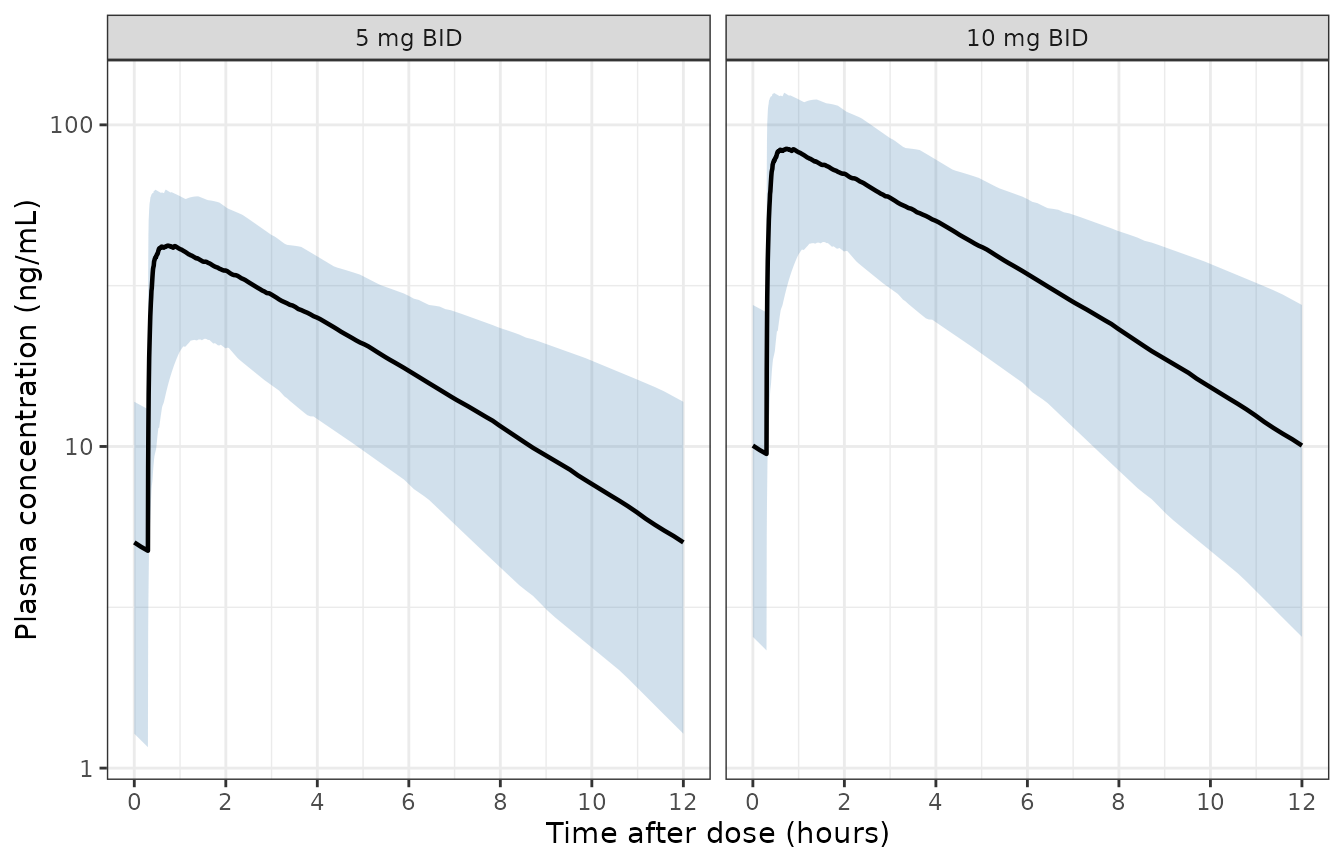

Replicates Figure 2 of Xie 2019: simulated concentration-time percentiles over a steady-state dosing interval, by dose group.

PKNCA validation at steady state

conc_data <- sim |>
  dplyr::filter(!is.na(Cc)) |>
  dplyr::select(id, treatment, time, Cc)

# Defensive interval-start anchor: every subject must have a record at exactly
# the start of the NCA interval, or PKNCA warns and the AUC is taken from the
# first available sample instead.
anchor_count <- conc_data |>
  dplyr::filter(time == t_ss) |>
  dplyr::count(treatment, id)
stopifnot(nrow(anchor_count) == 2 * n_sub, all(anchor_count$n == 1))

dose_data <- sim |>
  dplyr::distinct(treatment, id, dose) |>
  dplyr::mutate(time = t_ss)

conc_obj <- PKNCA::PKNCAconc(
  conc_data, Cc ~ time | treatment + id, concu = "ng/mL", timeu = "h"
)
dose_obj <- PKNCA::PKNCAdose(
  dose_data, dose ~ time | treatment + id, route = "extravascular", duration = 0
)

intervals <- data.frame(
  start = t_ss, end = t_ss + tau,
  cmax = TRUE, tmax = TRUE, cmin = TRUE, auclast = TRUE, cav = TRUE, half.life = TRUE
)

nca <- PKNCA::pk.nca(PKNCA::PKNCAdata(conc_obj, dose_obj, intervals = intervals))
nca_res <- as.data.frame(nca$result)

Simulated steady-state exposure

nca_summary <- nca_res |>
  dplyr::filter(PPTESTCD %in% c("cmax", "tmax", "cmin", "auclast", "cav", "half.life")) |>
  dplyr::group_by(treatment, PPTESTCD) |>
  dplyr::summarise(
    Median = median(PPORRES), P10 = quantile(PPORRES, 0.1),
    P90 = quantile(PPORRES, 0.9), .groups = "drop"
  ) |>
  dplyr::mutate(PPTESTCD = factor(
    PPTESTCD,
    levels = c("cmax", "tmax", "cmin", "cav", "auclast", "half.life"),
    labels = c("Cmax,ss (ng/mL)", "Tmax (h)", "Cmin,ss (ng/mL)",
               "Cavg,ss (ng/mL)", "AUC(0-tau) (ng*h/mL)", "t1/2 (h)")
  )) |>
  dplyr::arrange(treatment, PPTESTCD)

nca_summary |>
  dplyr::rename("Dose group" = treatment, "NCA parameter" = PPTESTCD,
                "10th percentile" = P10, "90th percentile" = P90) |>
  knitr::kable(digits = 2)

Dose group	NCA parameter	Median	10th percentile	90th percentile
5 mg BID	Cmax,ss (ng/mL)	45.63	27.71	60.90
5 mg BID	Tmax (h)	0.63	0.33	2.34
5 mg BID	Cmin,ss (ng/mL)	4.74	1.72	10.10
5 mg BID	Cavg,ss (ng/mL)	18.83	11.60	26.88
5 mg BID	AUC(0-tau) (ng*h/mL)	226.01	139.26	322.61
5 mg BID	t1/2 (h)	3.45	2.50	4.61
10 mg BID	Cmax,ss (ng/mL)	91.26	55.42	121.79
10 mg BID	Tmax (h)	0.63	0.33	2.34
10 mg BID	Cmin,ss (ng/mL)	9.48	3.44	20.21
10 mg BID	Cavg,ss (ng/mL)	37.67	23.21	53.77
10 mg BID	AUC(0-tau) (ng*h/mL)	452.02	278.52	645.21
10 mg BID	t1/2 (h)	3.45	2.50	4.61

Comparison against the analytic reference patient

Xie 2019 does not print an NCA table – its exposure statements are ratios (Figure 3) rather than absolute Cmax / AUC values. The natural reference is therefore the closed-form steady-state solution for the paper’s own reference patient, which is an independent calculation from the ODE solve.

analytic_reference <- lapply(c(5, 10), function(dose) {
  ka <- 13.8; cl <- 20.4; v <- 110; kel <- cl / v; tlag <- 0.3
  tt <- seq(0, tau, length.out = 200001)
  cc <- ss_closed_form(tt, dose, ka, kel, v, tau, tlag)
  data.frame(
    treatment = paste(dose, "mg BID"),
    cmax = max(cc), cmin = min(cc),
    cav = 1000 * dose / cl / tau,
    auclast = 1000 * dose / cl,
    half.life = log(2) / kel
  )
}) |> dplyr::bind_rows()

simulated_reference <- lapply(c(5, 10), function(dose) {
  d <- ss_profile(dose)
  auc <- sum(diff(d$time) * (head(d$Cc, -1) + tail(d$Cc, -1)) / 2)
  data.frame(
    treatment = paste(dose, "mg BID"),
    cmax = max(d$Cc), cmin = min(d$Cc), cav = auc / tau,
    auclast = auc, half.life = log(2) * d$vc[1] / d$cl[1]
  )
}) |> dplyr::bind_rows()
#> ℹ omega/sigma items treated as zero: 'etalcl', 'etalka', 'etaruv'
#> ℹ omega/sigma items treated as zero: 'etalcl', 'etalka', 'etaruv'

nca_compare <- nlmixr2lib::ncaComparisonTable(
  simulated = simulated_reference,
  reference = analytic_reference,
  by = "treatment",
  params = c("cmax", "cmin", "cav", "auclast", "half.life"),
  tolerance_pct = 20,
  label_first_column = "NCA parameter"
)
knitr::kable(nca_compare)

NCA parameter	treatment	Reference	Simulated	% diff
Cmax	5 mg BID	48.1	48.1	-0.0%
Cmax	10 mg BID	96.3	96.3	-0.0%
Cmin	5 mg BID	5.58	5.58	+0.0%
Cmin	10 mg BID	11.2	11.2	+0.0%
AUClast	5 mg BID	245	245	+0.0%
AUClast	10 mg BID	490	490	+0.0%
t½	5 mg BID	3.74	3.74	+0.0%
t½	10 mg BID	3.74	3.74	+0.0%
Cavg	5 mg BID	20.4	20.4	+0.0%
Cavg	10 mg BID	40.8	40.9	+0.0%

rel <- abs(
  simulated_reference[, c("cmax", "cmin", "cav", "auclast", "half.life")] /
    analytic_reference[, c("cmax", "cmin", "cav", "auclast", "half.life")] - 1
)
stopifnot(max(as.matrix(rel)) < 1e-3)

Per-subject mass balance across the cohort

The CL/F * AUC(0-tau) = Dose identity holds for every individual, not just the typical one, so it can be asserted across the whole cohort. The residual spread here is trapezoidal-integration error on the sharp absorption peak, not model error.

mass_balance <- nca_res |>
  dplyr::filter(PPTESTCD == "auclast") |>
  dplyr::left_join(individual_params, by = c("treatment", "id")) |>
  dplyr::left_join(dplyr::distinct(sim, treatment, id, dose), by = c("treatment", "id")) |>
  dplyr::mutate(pct_diff = 100 * (cl * PPORRES / 1000 / dose - 1))

cat(sprintf(
  "CL/F * AUC(0-tau) / Dose - 1: median %.4f%%, 90th percentile of |.| %.4f%%, max |.| %.4f%%\n",
  median(mass_balance$pct_diff),
  quantile(abs(mass_balance$pct_diff), 0.9),
  max(abs(mass_balance$pct_diff))
))
#> CL/F * AUC(0-tau) / Dose - 1: median -0.0002%, 90th percentile of |.| 0.0027%, max |.| 1.6487%

# Asserted on the centre and a robust quantile rather than on the maximum: the
# worst subject is whichever one happened to draw the slowest absorption, which
# is not reproducible across rxode2 versions or thread counts.
stopifnot(
  abs(median(mass_balance$pct_diff)) < 0.1,
  quantile(abs(mass_balance$pct_diff), 0.9) < 0.5
)

Dose proportionality

The model is linear, so simulating the same 200 subjects at 5 and 10 mg must give a 2-fold exposure ratio for every subject. Because the preceding chunk established that both arms use identical individual parameters, the only thing separating the ratio from exactly 2 is the ODE solver’s relative tolerance, so this takes a tight bound (observed: median exactly 2, worst subject within 3e-5).

ratios <- nca_res |>
  dplyr::filter(PPTESTCD %in% c("cmax", "cmin", "auclast", "cav")) |>
  dplyr::left_join(dplyr::distinct(sim, treatment, id, dose), by = c("treatment", "id")) |>
  dplyr::select(id, dose, PPTESTCD, PPORRES) |>
  tidyr::pivot_wider(names_from = dose, values_from = PPORRES, names_prefix = "d") |>
  dplyr::mutate(ratio = d10 / d5)

ratios |>
  dplyr::group_by(PPTESTCD) |>
  dplyr::summarise(`Median 10 mg / 5 mg ratio` = median(ratio),
                   `Max deviation from 2` = max(abs(ratio - 2)), .groups = "drop") |>
  dplyr::rename("NCA parameter" = PPTESTCD) |>
  knitr::kable(digits = 8)

NCA parameter	Median 10 mg / 5 mg ratio	Max deviation from 2
auclast	2	7.130e-06
cav	2	7.130e-06
cmax	2	1.350e-06
cmin	2	2.467e-05


stopifnot(max(abs(ratios$ratio - 2)) < 1e-3)

Replicating Figure 3 (covariate impact on AUC and Cmax)

Figure 3 of Xie 2019 is a forest plot of the change in steady-state AUC and Cmax relative to the reference patient. Because CL/F and V/F are deterministic functions of the covariates, the point estimates are reproduced exactly; the confidence intervals in the published figure come from 1,000 nonparametric bootstrap runs and are not reproducible from the point estimates alone, so only the point estimates are shown.

scenarios <- list(
  "Age 18 y" = list(AGE = 18), "Age 80 y" = list(AGE = 80),
  "BWT 61 kg" = list(WT = 61), "BWT 109 kg" = list(WT = 109),
  "BCCL 50 mL/min" = list(CRCL_BASE = 50), "BCCL 60 mL/min" = list(CRCL_BASE = 60),
  "BCRP 3.0 mg/dL" = list(CRP = 3.0), "Female" = list(SEXF = 1),
  "Non-Hispanic" = list(RACE_HISPANIC = 0), "Black" = list(RACE_BLACK = 1),
  "Asian" = list(RACE_ASIAN = 1), "Other race" = list(RACE_OTHER = 1)
)

ss_metrics <- function(overrides) {
  ev <- rxode2::et(amt = 5, cmt = "depot", ii = tau, addl = n_load) |>
    rxode2::et(t_ss + obs_times, cmt = "central")
  d <- rxode2::rxSolve(tv, with_covariates(ev, overrides),
                       returnType = "data.frame", maxsteps = 100000L)
  c(AUC = sum(diff(d$time) * (head(d$Cc, -1) + tail(d$Cc, -1)) / 2), Cmax = max(d$Cc))
}

ref_metrics <- ss_metrics(list())
#> ℹ omega/sigma items treated as zero: 'etalcl', 'etalka', 'etaruv'
forest <- lapply(names(scenarios), function(nm) {
  m <- ss_metrics(scenarios[[nm]])
  data.frame(Scenario = nm, Metric = c("AUC(0-tau)", "Cmax"),
             Ratio = 100 * as.numeric(m / ref_metrics))
}) |> dplyr::bind_rows()
#> ℹ omega/sigma items treated as zero: 'etalcl', 'etalka', 'etaruv'
#> ℹ omega/sigma items treated as zero: 'etalcl', 'etalka', 'etaruv'
#> ℹ omega/sigma items treated as zero: 'etalcl', 'etalka', 'etaruv'
#> ℹ omega/sigma items treated as zero: 'etalcl', 'etalka', 'etaruv'
#> ℹ omega/sigma items treated as zero: 'etalcl', 'etalka', 'etaruv'
#> ℹ omega/sigma items treated as zero: 'etalcl', 'etalka', 'etaruv'
#> ℹ omega/sigma items treated as zero: 'etalcl', 'etalka', 'etaruv'
#> ℹ omega/sigma items treated as zero: 'etalcl', 'etalka', 'etaruv'
#> ℹ omega/sigma items treated as zero: 'etalcl', 'etalka', 'etaruv'
#> ℹ omega/sigma items treated as zero: 'etalcl', 'etalka', 'etaruv'
#> ℹ omega/sigma items treated as zero: 'etalcl', 'etalka', 'etaruv'
#> ℹ omega/sigma items treated as zero: 'etalcl', 'etalka', 'etaruv'
forest$Scenario <- factor(forest$Scenario, levels = rev(names(scenarios)))

ggplot(forest, aes(x = Ratio, y = Scenario, colour = Metric)) +
  geom_vline(xintercept = 100, linetype = 1, colour = "grey40") +
  geom_vline(xintercept = c(80, 125), linetype = 3, colour = "grey60") +
  geom_point(position = position_dodge(width = 0.6), size = 2.2) +
  labs(x = "Change relative to the reference patient (%)", y = NULL, colour = NULL) +
  theme_bw() + theme(legend.position = "top")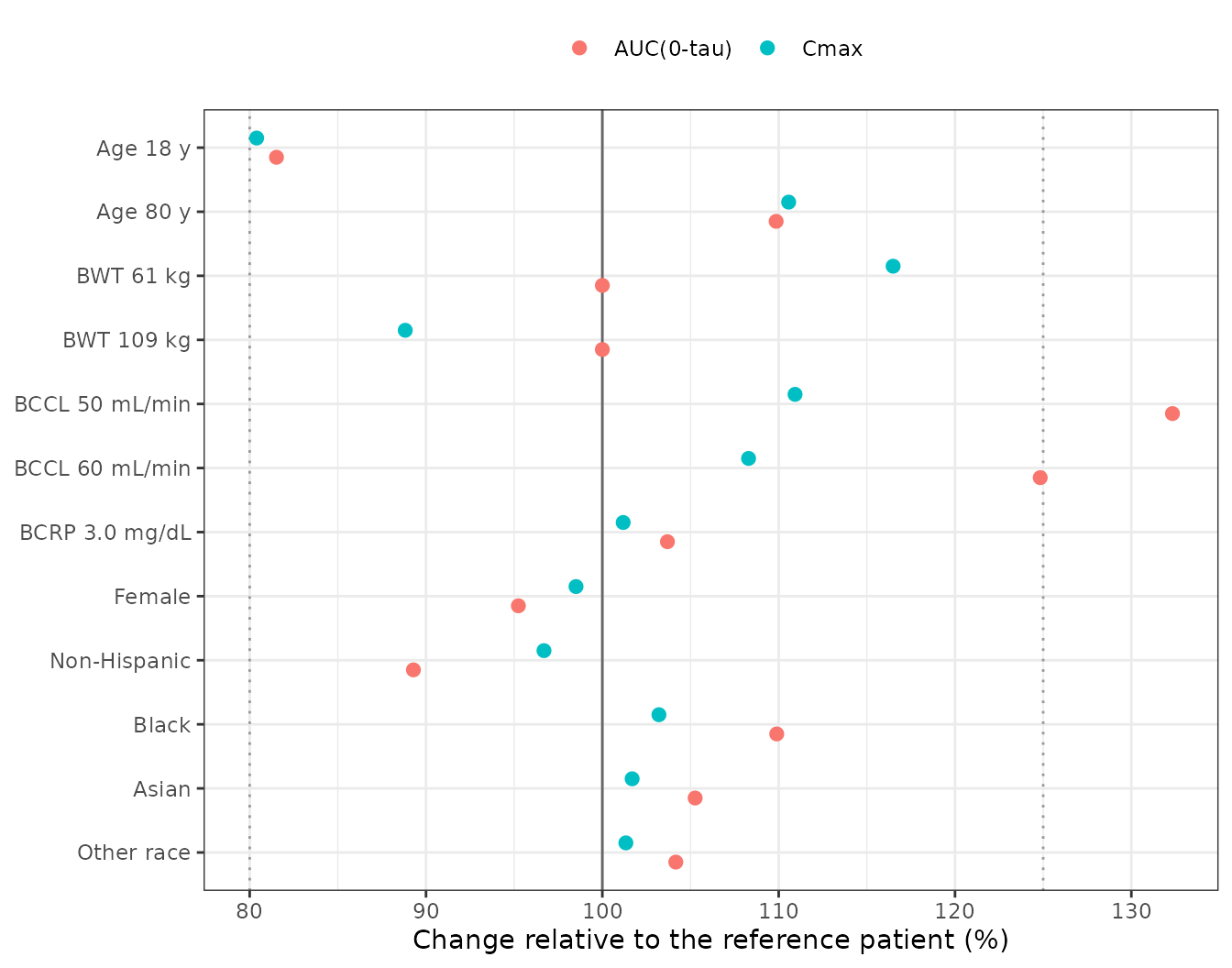

Replicates the point estimates of Figure 3 of Xie 2019: steady-state AUC and Cmax relative to the reference patient (White, male, Hispanic, 83.3 kg, 50 years, BCRP 0.49 mg/dL, BCCL 120 mL/min).

The paper states that, with the exception of BCCL, the AUC and Cmax point estimates span 88-110% and 89-116% of the reference values respectively, and that the BCCL 50 mL/min scenario raises AUC by 32%. Those two statements are checked below. Note that the 88-110% / 89-116% bands are the paper’s summary of the scenarios plotted in Figure 3, which uses percentile-based age and weight values rather than the full observed range; the check therefore excludes the age-18 extreme, which is outside the range Figure 3 plots.

bccl50_auc <- forest$Ratio[forest$Scenario == "BCCL 50 mL/min" & forest$Metric == "AUC(0-tau)"]
cat(sprintf("AUC at BCCL 50 mL/min: %.1f%% of reference (paper: 132%%)\n", bccl50_auc))
#> AUC at BCCL 50 mL/min: 132.3% of reference (paper: 132%)
stopifnot(abs(bccl50_auc - 132) < 1)

plotted <- !(forest$Scenario %in% c("Age 18 y", "BCCL 50 mL/min", "BCCL 60 mL/min"))
auc_band <- range(forest$Ratio[plotted & forest$Metric == "AUC(0-tau)"])
cmax_band <- range(forest$Ratio[plotted & forest$Metric == "Cmax"])
cat(sprintf("AUC band %.0f-%.0f%% (paper: 88-110%%); Cmax band %.0f-%.0f%% (paper: 89-116%%)\n",
            auc_band[1], auc_band[2], cmax_band[1], cmax_band[2]))
#> AUC band 89-110% (paper: 88-110%); Cmax band 89-116% (paper: 89-116%)
stopifnot(auc_band[1] > 85, auc_band[2] < 115, cmax_band[1] > 85, cmax_band[2] < 120)

Assumptions and deviations

IIV percent-to-variance convention (material). Table 3 reports IIV as a percent but never states whether it is 100 * sqrt(omega^2) or the exact log-normal CV 100 * sqrt(exp(omega^2) - 1). The model uses the first, the standard NONMEM / PsN reporting convention, so omega^2 = (IIV% / 100)^2. This is immaterial for CL/F (31.7% CV gives omega^2 of 0.100 either way to within 5%) but material for Ka: at 198%, the two readings give omega^2 of 3.92 and 1.59 respectively. Nothing in the paper adjudicates this, and no published NCA table exists to settle it empirically. Users who need the absorption-variability tail specifically should be aware that the packaged value is the wider of the two readings.
Ethnicity polarity. The paper’s reference category for ethnicity is the Hispanic group, and Table 3 reports a single factor (1.12) for non-Hispanic patients. The canonical covariate column RACE_HISPANIC keeps its register direction (1 = Hispanic), and the effect is applied through (1 - RACE_HISPANIC) in model(). A user supplying data coded the other way round will get the effect backwards.
Categorical coefficients are rounded in the source. Table 3 prints the sex and ethnicity multiplicative factors to two decimals (1.05, 1.12) while the Results prose quotes 5.4% and 12.3%, implying unrounded estimates of about 1.054 and 1.123. The packaged model uses the Table 3 values, which is why those two rows of the covariate-impact table are off by 0.3-0.4 percentage points.
Cohort covariate distributions are assumed. Table 2 reports mean, SD and range only. The virtual cohort draws truncated normals matched to the reported mean and SD, clipped at the reported range. BCRP in particular is strongly right-skewed in reality (mean 1.1, SD 2.0, max 16.4), so a truncated normal understates its tail; the BCRP effect on CL/F is negligible (exponent -0.02) so this has no material consequence for exposure. Covariates are also drawn independently, whereas weight, sex and creatinine clearance are correlated in the real cohort.
The 65.8% IIV on the residual magnitude is carried as etaruv. This eta has no paired fixed-effect parameter named ruv, so checkModelConventions() emits one warning about it. The name follows the existing Ooi_2026_elafibranor precedent for an eta on the residual-error magnitude; the alternative – pairing it to one of the two TAD-specific propSd parameters – would misrepresent a single variance component that the paper shares across both strata.
The body-weight effect on CL/F is retained at a fixed zero. It has no numerical effect; it is kept so the authors’ full covariate structure is visible in the model file rather than silently pruned.
No bioavailability parameter. The model is parameterized in apparent clearance and apparent volume, so F is folded into both and is not separately identifiable. Absolute exposures are only meaningful for oral dosing.
Bootstrap confidence intervals are not reproduced. Figure 3’s intervals come from 1,000 nonparametric bootstrap runs; only point estimates are reproduced here.
Patient-count arithmetic in the source. Table 1’s per-arm counts sum to 687 treatment-group assignments across the two studies while the Results state 650 patients with sufficient data for analysis. The paper does not reconcile the difference; 650 is used as the population size since that is the analysis dataset.
Renal-impairment dosing is out of scope. The paper notes that dose adjustments for renal impairment were derived from a separate phase 1 study, not from this model, and there were no patients with BCCL below 49 mL/min in the analysis dataset. Extrapolating the BCCL power function below that value is not supported by these data.

Session info

sessionInfo()
#> R version 4.6.1 (2026-06-24)
#> Platform: x86_64-pc-linux-gnu
#> Running under: Ubuntu 24.04.5 LTS
#> 
#> Matrix products: default
#> BLAS:   /usr/lib/x86_64-linux-gnu/openblas-pthread/libblas.so.3 
#> LAPACK: /usr/lib/x86_64-linux-gnu/openblas-pthread/libopenblasp-r0.3.26.so;  LAPACK version 3.12.0
#> 
#> locale:
#>  [1] LC_CTYPE=C.UTF-8       LC_NUMERIC=C           LC_TIME=C.UTF-8       
#>  [4] LC_COLLATE=C.UTF-8     LC_MONETARY=C.UTF-8    LC_MESSAGES=C.UTF-8   
#>  [7] LC_PAPER=C.UTF-8       LC_NAME=C              LC_ADDRESS=C          
#> [10] LC_TELEPHONE=C         LC_MEASUREMENT=C.UTF-8 LC_IDENTIFICATION=C   
#> 
#> time zone: UTC
#> tzcode source: system (glibc)
#> 
#> attached base packages:
#> [1] stats     graphics  grDevices utils     datasets  methods   base     
#> 
#> other attached packages:
#> [1] ggplot2_4.0.3         tidyr_1.3.2           dplyr_1.2.1          
#> [4] rxode2_5.1.8          PKNCA_0.12.1          nlmixr2lib_0.3.2.9000
#> 
#> loaded via a namespace (and not attached):
#>  [1] gtable_0.3.6        xfun_0.61           bslib_0.12.0       
#>  [4] rxode2lincmt_0.1.0  lattice_0.22-9      vctrs_0.7.3        
#>  [7] tools_4.6.1         generics_0.1.4      parallel_4.6.1     
#> [10] tibble_3.3.1        symengine_0.2.13    pkgconfig_2.0.3    
#> [13] data.table_1.18.6.1 checkmate_2.3.4     RColorBrewer_1.1-3 
#> [16] S7_0.2.2            desc_1.4.3          lifecycle_1.0.5    
#> [19] compiler_4.6.1      farver_2.1.2        textshaping_1.0.5  
#> [22] fontawesome_0.5.3   htmltools_0.5.9     sys_3.4.3          
#> [25] sass_0.4.10         yaml_2.3.12         pillar_1.11.1      
#> [28] pkgdown_2.2.1       crayon_1.5.3        jquerylib_0.1.4    
#> [31] whisker_0.4.1       openssl_2.4.2       cachem_1.1.0       
#> [34] nlme_3.1-169        tidyselect_1.2.1    digest_0.6.39      
#> [37] lotri_1.0.5         purrr_1.2.2         labeling_0.4.3     
#> [40] rxode2ll_2.0.18     fastmap_1.2.0       grid_4.6.1         
#> [43] cli_3.6.6           dparser_1.3.1-13    magrittr_2.0.5     
#> [46] withr_3.0.3         scales_1.4.0        backports_1.5.1    
#> [49] rmarkdown_2.32      otel_0.2.0          askpass_1.2.1      
#> [52] ragg_1.5.2          memoise_2.0.1       evaluate_1.0.5     
#> [55] knitr_1.52          rex_1.2.2           PreciseSums_0.7    
#> [58] rlang_1.3.0         downlit_0.4.5       Rcpp_1.1.2         
#> [61] glue_1.8.1          xml2_1.6.0          jsonlite_2.0.0     
#> [64] R6_2.6.1            systemfonts_1.3.2   fs_2.1.0