Palbociclib neutropenia (Le Marouille 2021)

Model and source

Le Marouille et al. (2021) modelled oral palbociclib pharmacokinetics and the time course of absolute neutrophil counts (ANC) in women treated for breast cancer in routine care at a French cancer centre. Palbociclib concentrations came from routine therapeutic drug monitoring (mostly one sample per patient) and ANC from the patient files over up to one year of treatment.

The population PK model is one-compartment with first-order absorption, an absorption lag time and first-order elimination. The sparse design could not support estimating V/F or the lag time, so both were fixed to the values of the earlier palbociclib model from the same centre (Royer 2021). Apparent clearance increases with Cockcroft-Gault creatinine clearance (CRCL) and decreases with serum alkaline phosphatase (ALP). The PK/PD model is Friberg’s semi-mechanistic myelosuppression model with a linear drug effect on proliferation. Baseline ANC increases with age. The PK/PD model was fitted sequentially: each patient’s individual PK parameters entered it as regressors. The packaged model combines both layers, so a simulation draws the PK random effect together with the PD random effects.

• Citation: Le Marouille A, Petit E, Kaderbhai C, Desmoulins I, Hennequin A, Mayeur D, Fumet JD, Ladoire S, Tharin Z, Ayati S, Ilie S, Royer B, Schmitt A. (2021). Pharmacokinetic/Pharmacodynamic Model of Neutropenia in Real-Life Palbociclib-Treated Patients. Pharmaceutics 13(10):1708. doi:10.3390/pharmaceutics13101708. V/F and Tlag were fixed to the values of Royer B et al. (2021) Population Pharmacokinetics of Palbociclib in a Real-World Situation. Pharmaceuticals 14(3):181. doi:10.3390/ph14030181.
• Article: https://doi.org/10.3390/pharmaceutics13101708 (open access)
• Supplement: https://www.mdpi.com/article/10.3390/pharmaceutics13101708/s1 (diagnostic figures only: NPC, NPDE and prediction-corrected VPC)

The paper’s first author is Alexandre Le Marouille. The model file uses the stem Marouille, which follows the journal’s own citation line (“Marouille, A.L.”).

Population

The popPK analysis used 181 plasma concentrations from 143 women (108 with one sample, 32 with two and 3 with three, each treated as an independent individual). Samples were drawn 0.9-197.25 h after the last dose, between day 1 and day 28 of a cycle, at doses of 125 mg (127 samples), 100 mg (38) or 75 mg (16) once daily, 21 days on and 7 days off. The PK/PD analysis used 1508 ANC from 128 of these patients (3-41 per patient) over up to 13 cycles.

Table 1 of the paper (popPK cohort / PK/PD cohort, median and range):

Characteristic	popPK (n = 143)	PK/PD (n = 128)
Age (years)	69 (40-92)	63 (40-92)
Weight (kg)	67 (37-140)	66 (37-140)
Serum creatinine (umol/L)	68.0 (31.0-301.8)	68.0 (31-169.7)
Cockcroft-Gault CRCL (mL/min)	71.6 (22.1-282.3)	73.5 (22.1-282.3)
ALP (U/L)	89 (11-819)	81 (11-644)
Albumin (g/L)	39.9 (20.0-48.0)	39.0 (20.0-48.0)

All patients were women. Concurrent hormonotherapy was letrozole in 49.6%, fulvestrant in 33.6% and another agent in 9.8% of the popPK cohort (Table 2).

Source trace

Model element	Value	Source
One-compartment PK, first-order absorption with lag	–	Section 3.2
lka	0.187 /h	Table 3, final model
lcl	57.13 L/h	Table 3, final model
lvc (fixed)	1580 L	Table 3; fixed to Royer 2021 (Section 3.2)
ltlag (fixed)	0.658 h	Table 3 (“T lag (h) (fix)”)
e_crcl_cl, centring value	0.44, 71.6 mL/min	Table 3
e_alp_cl, centring value	-0.14, 88.6 U/L	Table 3
Power covariate form (COV / COVmed)^beta	–	Section 2.6, Equation 1
etalcl	32.6% CV	Table 3
CV to variance, CV = sqrt(exp(omega^2) - 1)	–	Section 2.5
addSd	13.84 ug/L	Table 3
Friberg chain (PROL, 3 transits, CIRC), ktr = 4 / MTT, kprol = ktr = kcirc	–	Section 2.4, Figure 1
Drug effect E_D = C * Slope, feedback (CIRC0 / CIRC)^gamma	–	Figure 1
All compartments start at Base	–	Section 2.4
lcirc0	2.92 G/L	Table 4, final model
lslope	0.0011 L/ug	Table 4
lmtt	5.29 days (126.96 h)	Table 4
lgamma	0.103	Table 4
e_age_circ0, centring value	0.465, 63.7 years	Table 4
etalcirc0, etalslope, etalmtt	29.6%, 28.8%, 17.9% CV	Table 4
expSd_ANC (additive on log ANC)	0.34	Table 4; Section 2.4

Virtual patients and dosing

The label regimen is 125 mg once daily for 21 days of each 28-day cycle. The helper below builds a four-cycle event table (100 days, the horizon of the paper’s Figure 3 simulations). The model has two endpoints (Cc and ANC), so observation rows carry dvid = 1; both outputs come back as columns.

dose_times <- function(n_cycles = 4) {
  unlist(lapply(seq_len(n_cycles) - 1, function(cyc) cyc * 28 * 24 + (0:20) * 24))
}
make_events <- function(ids, dose_mg = 125, obs_times = seq(0, 100 * 24, by = 6)) {
  do.call(rbind, lapply(ids, function(i) {
    rbind(
      data.frame(id = i, time = dose_times(), amt = dose_mg, evid = 1L, cmt = "depot", dvid = NA_integer_),
      data.frame(id = i, time = obs_times, amt = 0, evid = 0L, cmt = NA_character_, dvid = 1L)
    )
  })) |>
    dplyr::arrange(id, time, dplyr::desc(evid))
}
mod <- readModelDb("Marouille_2021_palbociclib")
mod_typ <- rxode2::zeroRe(mod)
#> ℹ parameter labels from comments will be replaced by 'label()'

Pharmacokinetics

Typical steady state

Day 21 of the first cycle is the paper’s reference for the steady-state trough (CresSS). At the median covariates (CRCL 71.6 mL/min, ALP 88.6 U/L) the typical CL/F is 57.13 L/h.

doses <- c(75, 100, 125)
tau <- 24
ev_pk <- do.call(rbind, lapply(seq_along(doses), function(k) {
  make_events(k, dose_mg = doses[k], obs_times = sort(unique(c(seq(0, 504, by = 0.25)))))
})) |>
  dplyr::mutate(CRCL = 71.6, ALP = 88.6, AGE = 63.7)
# Tight tolerances so the closed-form check below tests the model, not the
# solver's default relative tolerance of 1e-6.
sim_pk <- rxode2::rxSolve(mod_typ, ev_pk, returnType = "data.frame", atol = 1e-10, rtol = 1e-10) |>
  as.data.frame() |>
  dplyr::mutate(dose = doses[id], treatment = paste(dose, "mg QD"))
#> ℹ omega/sigma items treated as zero: 'etalcl', 'etalcirc0', 'etalslope', 'etalmtt'
#> Warning: multi-subject simulation without without 'omega'

ggplot(sim_pk, aes(time / 24, Cc, colour = treatment)) +
  geom_line() +
  labs(x = "Day of cycle", y = "Palbociclib (ug/L)", colour = NULL) +
  theme_bw()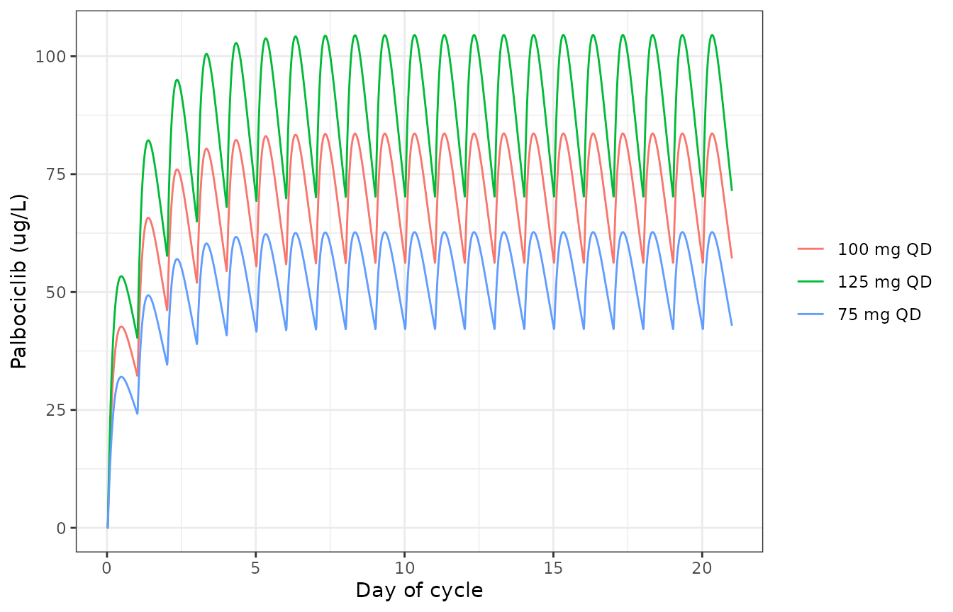

Typical palbociclib concentration over the first 21 days of a cycle at the median covariates.

Closed-form check

The steady-state one-compartment solution with a lag is evaluated at (t - tlag) %% tau. After 20 doses the non-steady-state remainder is exp(-kel * 480), about 3e-8, so the solve and the formula must agree closely.

p <- list(ka = 0.187, cl = 57.13, vc = 1580, tlag = 0.658)
kel <- p$cl / p$vc
css <- function(t, dose) {
  tp <- (t - p$tlag) %% tau
  1000 * dose * p$ka / (p$vc * (p$ka - kel)) *
    (exp(-kel * tp) / (1 - exp(-kel * tau)) - exp(-p$ka * tp) / (1 - exp(-p$ka * tau)))
}
last_int <- sim_pk |>
  dplyr::filter(time >= 480 + p$tlag + 0.1, time <= 504) |>
  dplyr::mutate(Cc_cf = css(time, dose))
rel_err <- max(abs(last_int$Cc / last_int$Cc_cf - 1))
rel_err
#> [1] 2.752781e-08
stopifnot(rel_err < 1e-6)

NCA over the day-21 dosing interval (PKNCA)

conc_ss <- sim_pk |>
  dplyr::filter(!is.na(Cc), time >= 480, time <= 504) |>
  dplyr::mutate(time = time - 480) |>
  dplyr::select(id, treatment, time, Cc)
dose_ss <- data.frame(id = seq_along(doses), treatment = paste(doses, "mg QD"), time = 0, amt = doses)

conc_obj <- PKNCA::PKNCAconc(conc_ss, Cc ~ time | treatment + id, concu = "ug/L", timeu = "h")
dose_obj <- PKNCA::PKNCAdose(dose_ss, amt ~ time | treatment + id, doseu = "mg")
intervals <- data.frame(
  start = 0, end = 24,
  cmax = TRUE, tmax = TRUE, ctrough = TRUE, auclast = TRUE, cav = TRUE
)
nca_res <- PKNCA::pk.nca(PKNCA::PKNCAdata(conc_obj, dose_obj, intervals = intervals))
nca_wide <- as.data.frame(nca_res$result) |>
  dplyr::select(treatment, PPTESTCD, PPORRES) |>
  tidyr::pivot_wider(names_from = PPTESTCD, values_from = PPORRES) |>
  dplyr::mutate(dose = as.numeric(sub(" mg QD", "", treatment)), auc_closed = 1000 * dose / p$cl)

nca_wide |>
  dplyr::select(treatment, cmax, tmax, ctrough, auclast, cav, auc_closed) |>
  dplyr::rename(
    "Dose" = treatment,
    "Cmax,ss (ug/L)" = cmax,
    "Tmax (h)" = tmax,
    "Ctrough,ss (ug/L)" = ctrough,
    "AUC0-24,ss (ug*h/L)" = auclast,
    "Cavg,ss (ug/L)" = cav,
    "Dose/CL (ug*h/L)" = auc_closed
  ) |>
  knitr::kable(digits = 1, caption = "Typical-value steady-state NCA on day 21 at the median covariates.")

Typical-value steady-state NCA on day 21 at the median covariates.

Dose	Cmax,ss (ug/L)	Tmax (h)	Ctrough,ss (ug/L)	AUC0-24,ss (ug*h/L)	Cavg,ss (ug/L)	Dose/CL (ug*h/L)
100 mg QD	83.6	8	57.1	1750.4	72.9	1750.4
125 mg QD	104.5	8	71.4	2188.0	91.2	2188.0
75 mg QD	62.7	8	42.9	1312.8	54.7	1312.8

auc_ratio <- nca_wide$auclast / nca_wide$auc_closed
auc_ratio
#> [1] 1.000012 1.000012 1.000012
# The trapezoid on a 0.25-h grid differs from the exact Dose/CL by well under 1%;
# a wrong clearance, dose or unit factor moves it by tens of percent.
stopifnot(all(abs(auc_ratio - 1) < 0.01))

Comparison with the published exposure groups

The paper reports no NCA table. Its Figure 5 splits the 127 patients who started at 125 mg into exposure quartiles, both on the single-dose AUC = Dose / CL computed from each patient’s individual clearance and on the estimated CresSS. The two middle groups meet at AUC 2.16 / 2.17 mgh/L and at CresSS 69 / 70 ug/L, so the cohort medians are about 2.165 mgh/L (2165 ug*h/L) and 69.5 ug/L. For a linear model the single-dose AUC(0-inf) equals AUC(0-24) at steady state, and a typical patient at the median covariates should sit close to the cohort median.

nca_125 <- as.data.frame(nca_res$result) |>
  dplyr::filter(treatment == "125 mg QD", PPTESTCD %in% c("auclast", "ctrough"))
reference_125 <- data.frame(treatment = "125 mg QD", auclast = 2165, ctrough = 69.5)
cmp <- ncaComparisonTable(
  nca_125, reference_125,
  by = "treatment",
  units = c(auclast = "ug*h/L", ctrough = "ug/L")
)
knitr::kable(cmp, caption = "Typical patient on 125 mg QD versus the medians implied by the Figure 5 quartile cut-points.")

Typical patient on 125 mg QD versus the medians implied by the Figure 5 quartile cut-points.

NCA parameter	treatment	Reference	Simulated	% diff
AUClast (ug*h/L)	125 mg QD	2160	2190	+1.1%
Ctrough (ug/L)	125 mg QD	69.5	71.4	+2.8%

sim_vals <- setNames(nca_125$PPORRES, nca_125$PPTESTCD)
stopifnot(
  abs(sim_vals[["auclast"]] / 2165 - 1) < 0.05,
  abs(sim_vals[["ctrough"]] / 69.5 - 1) < 0.05
)

The typical half-life is log(2) * V/F / (CL/F) = 19.2 h.

Pharmacodynamics

Figure 3: effect of each covariate on the ANC time course

Figure 3 of the paper simulates four cycles of 125 mg with every covariate at its median except one, which is set to an extreme of the PK/PD cohort (CRCL 22 or 279 mL/min, ALP 11 or 644 U/L, age 40 or 90 years), without inter-individual variability. The maintainers digitized the first-cycle nadir and the following rebound peak of each curve from the published raster figure.

scen <- data.frame(
  id = 1:7,
  panel = c("A-C", "A: CRCL", "A: CRCL", "B: ALP", "B: ALP", "C: age", "C: age"),
  scenario = c(
    "Median covariates", "CRCL 22 mL/min", "CRCL 279 mL/min",
    "ALP 11 U/L", "ALP 644 U/L", "Age 40 years", "Age 90 years"
  ),
  CRCL = c(71.6, 22, 279, 71.6, 71.6, 71.6, 71.6),
  ALP = c(88.6, 88.6, 88.6, 11, 644, 88.6, 88.6),
  AGE = c(63.7, 63.7, 63.7, 63.7, 63.7, 40, 90)
)
ev_fig3 <- make_events(scen$id) |>
  dplyr::left_join(scen[, c("id", "CRCL", "ALP", "AGE")], by = "id")
sim_fig3 <- rxode2::rxSolve(mod_typ, ev_fig3, returnType = "data.frame") |>
  as.data.frame() |>
  dplyr::left_join(scen[, c("id", "scenario")], by = "id")
#> ℹ omega/sigma items treated as zero: 'etalcl', 'etalcirc0', 'etalslope', 'etalmtt'
#> Warning: multi-subject simulation without without 'omega'

ggplot(sim_fig3, aes(time / 24, ANC, colour = scenario)) +
  geom_line() +
  scale_x_continuous(breaks = c(0, 21, 28, 49, 56, 77, 84, 100)) +
  coord_cartesian(ylim = c(0, 4)) +
  labs(x = "Time (days)", y = "ANC (G/L)", colour = NULL) +
  theme_bw()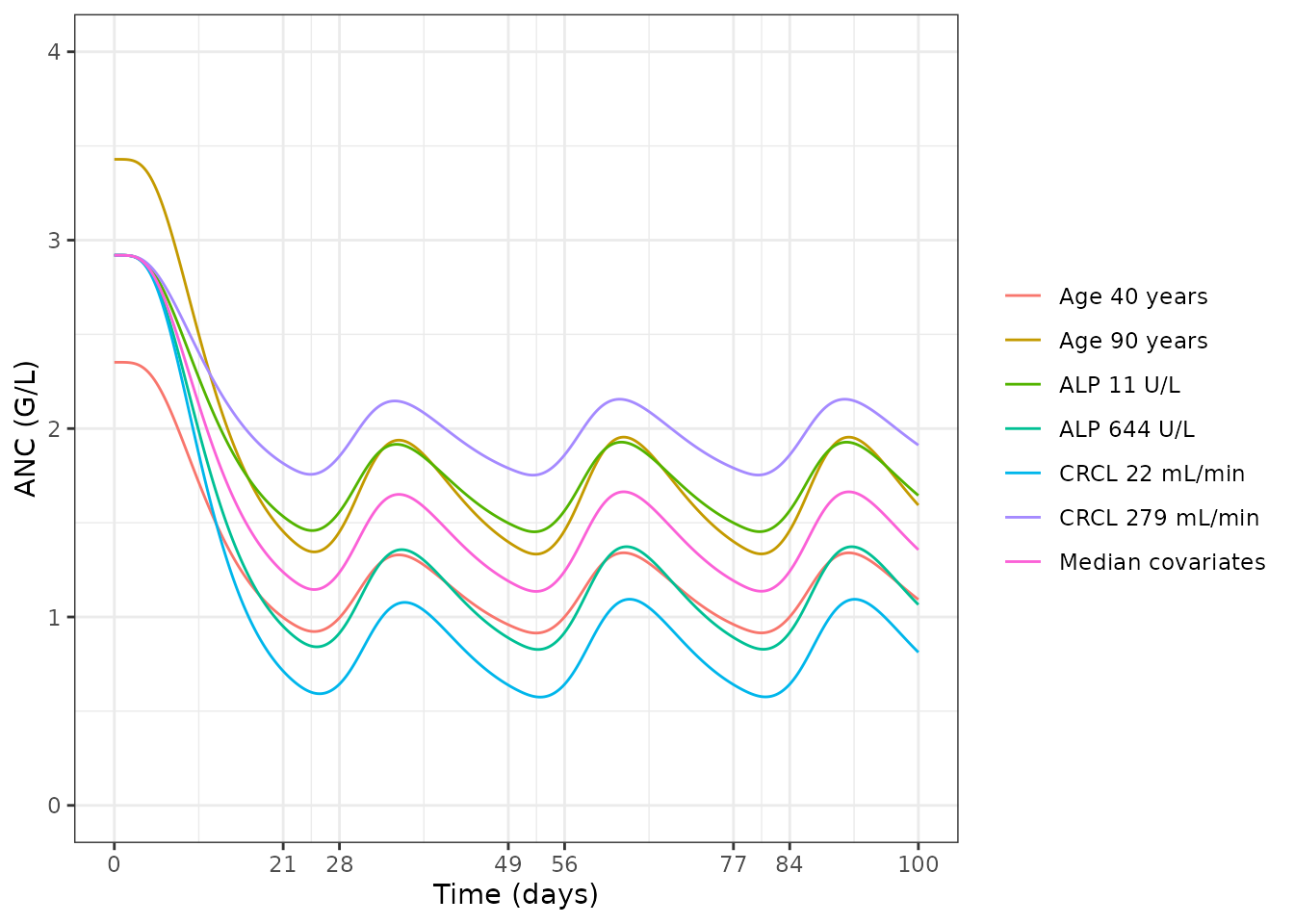

Replicates Figure 3 of Le Marouille 2021: typical ANC over four 28-day cycles of 125 mg (21 days on, 7 off).

digitized <- data.frame(
  scenario = scen$scenario,
  nadir_paper = c(1.12, 0.53, 1.76, 1.35, 0.79, 0.91, 1.32),
  peak_paper = c(1.62, 1.01, 2.15, 1.83, 1.31, 1.31, 1.90)
)
fig3_cmp <- sim_fig3 |>
  dplyr::group_by(scenario) |>
  dplyr::summarise(
    baseline = ANC[time == 0],
    nadir_model = min(ANC[time > 14 * 24 & time <= 30 * 24]),
    peak_model = max(ANC[time > 28 * 24 & time <= 45 * 24]),
    .groups = "drop"
  ) |>
  dplyr::inner_join(digitized, by = "scenario") |>
  dplyr::arrange(match(scenario, scen$scenario))
fig3_cmp |>
  dplyr::rename(
    "Scenario" = scenario,
    "Baseline (G/L)" = baseline,
    "Cycle-1 nadir, model" = nadir_model,
    "Cycle-1 nadir, Figure 3" = nadir_paper,
    "Rebound peak, model" = peak_model,
    "Rebound peak, Figure 3" = peak_paper
  ) |>
  knitr::kable(digits = 2, caption = "First-cycle nadir and following rebound peak (G/L): packaged model versus values digitized from Figure 3.")

First-cycle nadir and following rebound peak (G/L): packaged model versus values digitized from Figure 3.

Scenario	Baseline (G/L)	Cycle-1 nadir, model	Rebound peak, model	Cycle-1 nadir, Figure 3	Rebound peak, Figure 3
Median covariates	2.92	1.15	1.65	1.12	1.62
CRCL 22 mL/min	2.92	0.59	1.08	0.53	1.01
CRCL 279 mL/min	2.92	1.76	2.15	1.76	2.15
ALP 11 U/L	2.92	1.46	1.92	1.35	1.83
ALP 644 U/L	2.92	0.84	1.36	0.79	1.31
Age 40 years	2.35	0.92	1.33	0.91	1.31
Age 90 years	3.43	1.35	1.94	1.32	1.90

err <- abs(c(fig3_cmp$nadir_model - fig3_cmp$nadir_paper, fig3_cmp$peak_model - fig3_cmp$peak_paper))
med <- fig3_cmp[fig3_cmp$scenario == "Median covariates", ]
stopifnot(
  # The median-covariate curve is the anchor; digitization is good to ~0.02 G/L.
  abs(med$nadir_model - med$nadir_paper) < 0.06,
  abs(med$peak_model - med$peak_paper) < 0.06,
  # The age panel checks the power form of the age effect on Base directly.
  abs(fig3_cmp$baseline[fig3_cmp$scenario == "Age 40 years"] - 2.35) < 0.02,
  abs(fig3_cmp$baseline[fig3_cmp$scenario == "Age 90 years"] - 3.43) < 0.02,
  # Every curve: a wrong exponent sign or centring value moves these by > 0.3 G/L.
  max(err) < 0.15
)

The median-covariate, CRCL and age curves agree with the figure to within about 0.07 G/L. Both ALP curves sit about 0.05-0.11 G/L above the figure. The median curve they share matches, so the difference is specific to the ALP extremes; its source could not be identified from the paper.

Figure 4: risk of neutropenia against the steady-state trough

Figure 4 shows the proportion of 5000 simulated patients with a grade 3/4 (ANC < 1 G/L) or grade 4 (ANC < 0.5 G/L) nadir as a function of the estimated CresSS. The paper does not detail the protocol. It is reproduced here as follows. For each target CresSS the clearance giving that day-21 trough on 125 mg is solved from the closed form. Every virtual patient is given that clearance, and the PD random effects (Base, Slope, MTT) are drawn from Table 4. The nadir over 100 days (four cycles) is recorded without residual error. Age is at the median. The random effects are drawn in base R with a fixed seed and passed to the model as data, so the solve itself is deterministic. The cohort is 200 patients per CresSS value.

ctrough_ss <- function(cl) {
  k <- cl / p$vc
  1000 * 125 * p$ka / (p$vc * (p$ka - k)) *
    (exp(-k * (tau - p$tlag)) / (1 - exp(-k * tau)) - exp(-p$ka * (tau - p$tlag)) / (1 - exp(-p$ka * tau)))
}
cl_for_trough <- function(target) uniroot(function(cl) ctrough_ss(cl) - target, c(1, 2000))$root
stopifnot(abs(ctrough_ss(57.13) - sim_vals[["ctrough"]]) < 1e-3)

cress_grid <- c(40, 61, 80, 100, 120, 150, 200)
n_per <- 200
set.seed(20211016)
omega <- c(etalcirc0 = 0.08393, etalslope = 0.07965, etalmtt = 0.03153)
fig4_pat <- expand.grid(k = seq_len(n_per), cress = cress_grid) |>
  dplyr::mutate(
    id = dplyr::row_number(),
    etalcl = vapply(cress, function(x) log(cl_for_trough(x) / 57.13), numeric(1)),
    etalcirc0 = rnorm(dplyr::n(), 0, sqrt(omega[["etalcirc0"]])),
    etalslope = rnorm(dplyr::n(), 0, sqrt(omega[["etalslope"]])),
    etalmtt = rnorm(dplyr::n(), 0, sqrt(omega[["etalmtt"]]))
  )
ev_fig4 <- make_events(fig4_pat$id, obs_times = seq(0, 100 * 24, by = 12)) |>
  dplyr::left_join(fig4_pat[, c("id", "etalcl", "etalcirc0", "etalslope", "etalmtt")], by = "id") |>
  dplyr::mutate(CRCL = 71.6, ALP = 88.6, AGE = 63.7)
sim_fig4 <- rxode2::rxSolve(mod_typ, ev_fig4, returnType = "data.frame") |>
  as.data.frame()
#> ℹ omega/sigma items treated as zero: 'etalcl', 'etalcirc0', 'etalslope', 'etalmtt'
#> Warning: multi-subject simulation without without 'omega'
fig4_res <- sim_fig4 |>
  dplyr::group_by(id) |>
  dplyr::summarise(nadir = min(ANC), trough21 = Cc[time == 21 * 24], .groups = "drop") |>
  dplyr::left_join(fig4_pat[, c("id", "cress")], by = "id")
# The clearance back-solve lands every patient on its target day-21 trough
# (to the solver's default tolerance; a wrong back-solve misses by percent).
stopifnot(max(abs(fig4_res$trough21 / fig4_res$cress - 1)) < 1e-3)
risk <- fig4_res |>
  dplyr::group_by(cress) |>
  dplyr::summarise(g34_model = 100 * mean(nadir < 1), g4_model = 100 * mean(nadir < 0.5), .groups = "drop")

fig4_digitized <- data.frame(
  cress = cress_grid,
  g34_paper = c(11.8, 29.5, 49.4, 67.7, 81.2, 91.6, 97.8),
  g4_paper = c(0.0, 1.9, 7.8, 17.5, 32.0, 53.9, 79.7)
)
fig4_cmp <- dplyr::inner_join(risk, fig4_digitized, by = "cress")
fig4_cmp |>
  dplyr::rename(
    "CresSS (ug/L)" = cress,
    "Grade 3/4 risk, model (%)" = g34_model,
    "Grade 3/4 risk, Figure 4 (%)" = g34_paper,
    "Grade 4 risk, model (%)" = g4_model,
    "Grade 4 risk, Figure 4 (%)" = g4_paper
  ) |>
  knitr::kable(digits = 1, caption = "Risk of a grade 3/4 or grade 4 ANC nadir versus CresSS: packaged model (200 patients per row) versus values digitized from Figure 4.")

Risk of a grade 3/4 or grade 4 ANC nadir versus CresSS: packaged model (200 patients per row) versus values digitized from Figure 4.

CresSS (ug/L)	Grade 3/4 risk, model (%)	Grade 4 risk, model (%)	Grade 3/4 risk, Figure 4 (%)	Grade 4 risk, Figure 4 (%)
40	11.5	0.0	11.8	0.0
61	31.0	2.0	29.5	1.9
80	53.0	6.0	49.4	7.8
100	71.5	18.5	67.7	17.5
120	83.0	33.0	81.2	32.0
150	93.0	49.5	91.6	53.9
200	98.0	82.0	97.8	79.7

fig4_long <- fig4_cmp |>
  tidyr::pivot_longer(-cress, names_to = c("grade", "source"), names_sep = "_", values_to = "risk") |>
  dplyr::mutate(grade = ifelse(grade == "g34", "Grade 3/4", "Grade 4"))
ggplot(fig4_long, aes(cress, risk, colour = grade)) +
  geom_line(data = dplyr::filter(fig4_long, source == "model")) +
  geom_point(data = dplyr::filter(fig4_long, source == "paper")) +
  labs(x = "CresSS (ug/L)", y = "Cumulative risk of neutropenia (%)", colour = NULL) +
  theme_bw()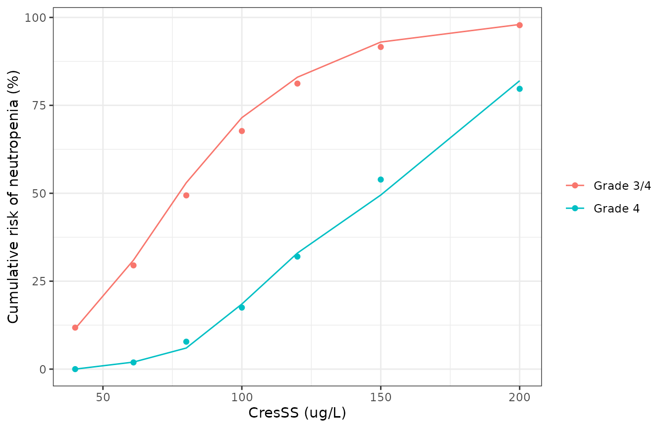

Replicates Figure 4 of Le Marouille 2021: cumulative risk of neutropenia against the steady-state trough (lines, packaged model; points, digitized from the figure).

stopifnot(
  # Section 3.4: 'At an estimated CresSS of 100 ug/L, a patient has an 18% risk
  # of developing grade 4 neutropenia'. The binomial SD at n = 200 is ~2.7 points.
  abs(fig4_cmp$g4_model[fig4_cmp$cress == 100] - 18) < 8,
  # Discussion: a CresSS of 61 ug/L gives about a 31% risk of grade 3 neutropenia.
  abs(fig4_cmp$g34_model[fig4_cmp$cress == 61] - 31) < 10,
  # Whole curve: a wrong Slope unit (1000-fold) or MTT unit (24-fold) gives 0% or 100%.
  median(abs(c(fig4_cmp$g34_model - fig4_cmp$g34_paper, fig4_cmp$g4_model - fig4_cmp$g4_paper))) < 5
)

Stochastic cohort at 125 mg

A cohort of 200 patients at the median covariates, with all random effects drawn from the model (PK and PD), shows the spread of ANC over four cycles. The paper’s prediction-corrected VPC (Supplementary Figure S4) is based on the observed data and is not reproduced here.

rxode2::rxSetSeed(2021)
ev_vpc <- make_events(1:200, obs_times = seq(0, 100 * 24, by = 24)) |>
  dplyr::mutate(CRCL = 71.6, ALP = 88.6, AGE = 63.7)
sim_vpc <- rxode2::rxSolve(mod, ev_vpc, returnType = "data.frame") |>
  as.data.frame()
#> ℹ parameter labels from comments will be replaced by 'label()'
vpc_sum <- sim_vpc |>
  dplyr::group_by(time) |>
  dplyr::summarise(
    p05 = quantile(ANC, 0.05), p50 = median(ANC), p95 = quantile(ANC, 0.95),
    .groups = "drop"
  )

ggplot(vpc_sum, aes(time / 24)) +
  geom_ribbon(aes(ymin = p05, ymax = p95), alpha = 0.25) +
  geom_line(aes(y = p50)) +
  geom_hline(yintercept = c(0.5, 1), linetype = "dashed") +
  scale_x_continuous(breaks = c(0, 21, 28, 49, 56, 77, 84, 100)) +
  labs(x = "Time (days)", y = "ANC (G/L)") +
  theme_bw()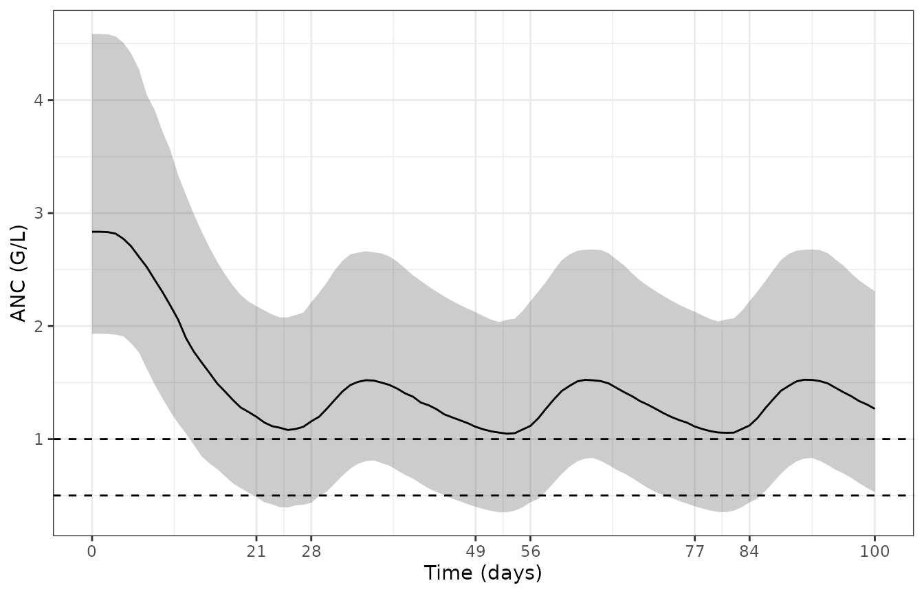

Simulated ANC (with residual error) for 200 patients on 125 mg at the median covariates: median and 5th-95th percentiles.

Assumptions and deviations

• Model factoring. The authors fitted the PK/PD model sequentially, with each patient’s individual PK parameters as fixed regressors. The packaged model contains both layers, so in a simulation the CL/F random effect is drawn together with the PD random effects. To reproduce a single patient, supply that patient’s etalcl (or covariates) as data.
• Covariate centring values. The centring values are the ones printed in the parameter tables: CRCL 71.6 mL/min, ALP 88.6 U/L (Table 1 gives 89) and age 63.7 years (Table 1 gives 63 for the PK/PD cohort). Missing covariates were imputed with the cohort median in the original analysis.
• Abstract versus tables. The Abstract quotes CL/F = 57.09 (with the unit printed as “L”) and 32.8% IIV. The Abstract and Discussion quote gamma = 0.102. The model uses the final-model estimates in Tables 3 and 4 (57.13 L/h, 32.6% and 0.103).
• Residual error. The PK error is additive (13.84 ug/L). The ANC error is additive on log-transformed ANC (Section 2.4) and is encoded as log-normal (lnorm) with SD 0.34.
• Linear drug effect. 1 - Slope * C is used as published. It would turn negative above 1/Slope = 909 ug/L, about four times the highest observed concentration (229 ug/L).
• Figure 4 protocol. The paper does not state how a patient was assigned a given CresSS or whether residual error entered the nadir. The protocol above (clearance back-solved from the target trough, PD random effects only, nadir over 100 days) reproduces the digitized curve closely.
• Units. ANC is in G/L (10^9 cells/L). MTT is converted from days to hours (5.29 x 24 = 126.96 h) so the model runs in hours throughout.
• Literature check. No erratum or correction was found on Europe PMC or the journal page (checked 2026-09-29).