Oxypurinol (Hishe 2023)
Source:vignettes/articles/Hishe_2023_oxypurinol.Rmd
Hishe_2023_oxypurinol.RmdModel and source
#> ℹ parameter labels from comments will be replaced by 'label()'- Citation: Hishe HZ, Stocker SL, Stamp LK, Dalbeth N, Merriman TR, Phipps-Green A, Wright DFB. The impact of genetic variability in urate transporters on oxypurinol pharmacokinetics. Clin Transl Sci. 2023 Mar;16(3):422-428. doi:10.1111/cts.13460
- Description: One-compartment population PK model for oxypurinol (the active metabolite of allopurinol) in adults with gout (Hishe 2023 Clin Transl Sci). Pooled analysis of five New Zealand studies (NONMEM 7.3, FOCEI): first-order absorption with Ka fixed at 0.993 1/h, one-compartment distribution and first-order elimination. Apparent oral clearance CL/F is power-scaled on Cockcroft-Gault creatinine clearance standardised to 70 kg (CRCL in L/h, reference 6 L/h), multiplicatively reduced by concomitant diuretic use (CONMED_DIURETIC) and increased in Pacific peoples (RACE_PACIFIC), and power-scaled on total body weight; apparent volume V/F is linearly weight-scaled. The dose entered into the model is allopurinol oral mg; the implicit 1:1 molar conversion to oxypurinol uses a 0.9 conversion factor and the allopurinol molecular weight 136.11 g/mol, so Cc is oxypurinol concentration in umol/L. Seven urate-transporter gene variants (ABCG2, SLC2A9, SLC17A1, SLC22A12, SLC22A11, ABCC4) were screened but none were retained in the final model. A separate combined additive + proportional residual error was estimated for each of the five studies.
- Article: https://doi.org/10.1111/cts.13460
The packaged model implements the Hishe 2023 final covariate model of
oxypurinol (the active metabolite of allopurinol) population
pharmacokinetics in adults with gout, pooled across five New Zealand
studies and fitted in NONMEM 7.3 (FOCE-I). The structural model is
one-compartment with first-order absorption (Ka fixed at 0.993 1/h) and
first-order elimination. Apparent oral clearance CL/F is power-scaled on
Cockcroft-Gault creatinine clearance standardised to 70 kg
(CRCL, in L/h, reference 6 L/h), reduced multiplicatively
by concomitant diuretic use (CONMED_DIURETIC), raised
multiplicatively in Pacific peoples (RACE_PACIFIC), and
power-scaled on total body weight (WT); apparent volume V/F
is linearly weight-scaled. A separate combined additive + proportional
residual error was estimated for each of the five studies, selected by
the STUDY_* indicator columns (Study 5 / Stamp 2017, the
largest sub-cohort, is the all-zeros reference). Seven urate-transporter
gene variants were screened but none were retained in the final
model.
The dose entered into the model is oral allopurinol in mg. Only
oxypurinol concentrations were measured, so bioavailability, the paper’s
0.9 allopurinol-to-oxypurinol conversion factor and the molar conversion
are absorbed into the apparent CL/F and V/F; the observation
Cc is oxypurinol concentration in umol/L (see Assumptions
for the molar-vs-mass reading of the 0.9 factor).
Population
Hishe 2023 fit the model to 2841 plasma oxypurinol concentrations from 300 adults with gout (264 male / 36 female; sex-female 12%) pooled across five New Zealand studies conducted in Christchurch and Auckland. The cohort was middle-aged to elderly (age range 23-86 years, median 61), heavy (total body weight range 51-186 kg, median 102 kg) and spanned a wide range of renal function (Cockcroft-Gault creatinine clearance 8-167 mL/min, median 63 mL/min). Allopurinol doses ranged 50-900 mg/day (median 300 mg/day). By ethnicity the cohort was 59% European / NZ European, 21% Pacific peoples, 16% Maori, 2% Chinese, 2% Indian and 1% Other; 37% were on a concomitant diuretic. The full demographic summary appears in Hishe 2023 Table S4; the transporter genotype distribution is in Table 1.
The same metadata is available programmatically via
readModelDb("Hishe_2023_oxypurinol")()$population.
Source trace
The per-parameter origin is recorded as an in-file comment next to
each ini() entry in
inst/modeldb/specificDrugs/Hishe_2023_oxypurinol.R. The
table below collects them in one place for review. All point estimates
are from Hishe 2023 Table 2 (“Final model” column); the structural
layout and covariate parameterisation are from the Results equations and
the Appendix S2 NONMEM control stream.
| Equation / parameter | Value | Source location |
|---|---|---|
lka (Ka) |
fixed(log(0.993)) | Table 2 row “ka”; Appendix S2 $THETA
0.993 FIX
|
lcl (CL/F) |
log(0.97) -> 0.97 L/h | Table 2 row “thetaCL”; bootstrap 0.97 [0.88-1.06] |
lvc (V/F) |
log(49) -> 49 L | Table 2 row “thetaV”; bootstrap 49 [43-54] |
e_crcl_cl (thetaRFexp) |
0.58 | Table 2 row “thetaRFexp”; bootstrap 0.58 [0.49-0.66] |
e_conmed_diuretic_cl (thetad) |
0.79 | Table 2 row “thetaddiuretic”; bootstrap 0.79 [0.74-0.85]; -21% on CL |
e_race_pacific_cl (thetae) |
1.25 | Table 2 row “thetaeethnicity”; bootstrap 1.25 [1.12-1.37]; +25% on CL |
e_wt_cl (thetaWTexp) |
0.34 | Table 2 row “thetaWTexp”; bootstrap 0.35 [0.17-0.53] |
e_wt_vc |
fixed(1.0) | Results equation V/F = thetaV * (WT/70); no Table 2
exponent row |
etalcl variance |
0.298^2 = 0.088804 | Table 2 row “omega CL CV%” = 29.8% (as log-SD; see Assumptions) |
etalvc variance |
0.413^2 = 0.170569 | Table 2 row “omega V CV%” = 41.3% |
etalcl x etalvc cov |
0.41 * sqrt(0.088804 * 0.170569) = 0.050464 | Table 2 row “Corr omega CL, omega V” = 0.41 |
etalka variance |
fixed(0.388) | Table 2 “omega Ka CV%” 62.3% (fixed); Appendix S2
$OMEGA 0.388 FIX
|
addSd_s1 / propSd_s1
|
fixed(0.0001) / 0.435 | Table 2 Study 1 residual error |
addSd_s2 / propSd_s2
|
10.0 / fixed(0.0001) | Table 2 Study 2 residual error |
addSd_s3 / propSd_s3
|
fixed(0.0001) / 0.422 | Table 2 Study 3 residual error |
addSd_s4 / propSd_s4
|
0.93 / 0.348 | Table 2 Study 4 residual error |
addSd_s5 / propSd_s5
|
fixed(0.0001) / 0.485 | Table 2 Study 5 residual error |
| CL/F equation | thetaCL * (CRCL/6)^0.58 * 0.79^DIURETIC * 1.25^PACIFIC * (WT/70)^0.34 |
Results covariate-model equation; Appendix S2 $PK
|
| V/F equation | thetaV * (WT/70) |
Results covariate-model equation |
ODE d/dt(depot)
|
-ka * depot |
One-compartment first-order absorption (Appendix S1 base model) |
ODE d/dt(central)
|
ka * depot - kel * central |
Same |
Observation Cc
|
0.9 * central / vc * 1000 / 136.11 |
0.9 conversion factor (Appendix S1) x molar conversion with allopurinol MW 136.11 |
Virtual cohort
Original observed concentration-time data are not publicly available. The vignette builds two virtual populations against which the packaged model is validated.
Cohort A – a representative pooled cohort (n = 200) with covariates sampled to approximate the Hishe 2023 Table S4 marginal distributions: log-normal body weight (median 102 kg), log-normal creatinine clearance (median 63 mL/min, i.e. 3.78 L/h standardised to 70 kg), 37% on a diuretic and 21% Pacific peoples. This cohort carries the model’s full between-subject and residual variability and is used for the steady-state VPC and the NCA.
Cohort B – covariate-effect strata (typical-value, random effects zeroed): a small set of one-at-a-time covariate contrasts used to confirm the Table 2 clearance covariate multipliers exactly.
All subjects receive once-daily oral allopurinol 300 mg (the cohort
median) for 14 days to reach approximate steady state; concentrations
are observed densely across the final dosing interval. All
STUDY_* indicators are left at 0, so the residual error is
that of Study 5 (Stamp 2017, the largest sub-cohort and the reference
level).
# `set.seed()` seeds R's RNG for the covariate draws below; it does NOT seed
# rxode2's per-thread simulation RNG, so the realised cohort differs across
# machines with different thread counts. Every assertion downstream is written
# to hold for any cohort the model can produce (centre + robust bounds), per
# the repository's vignette-assertion guidance.
set.seed(20230314)

mod_full    <- rxode2::rxode(readModelDb("Hishe_2023_oxypurinol"))
#> ℹ parameter labels from comments will be replaced by 'label()'
mod_typical <- rxode2::zeroRe(mod_full)
#> Warning: No sigma parameters in the model

dose_mg   <- 300    # cohort median allopurinol dose (mg/day)
tau       <- 24     # dosing interval (h)
n_doses   <- 14L    # 14 daily doses to reach steady state
n_per_arm <- 200L

ref_crcl <- 6       # L/h (normalisation standard = 100 mL/min/70 kg)
ref_wt   <- 70

# Log-normal covariate draws calibrated to the Table S4 medians and ranges.
# CRCL is stored in L/h standardised to 70 kg: the cohort median 63 mL/min
# corresponds to 63 * 0.06 = 3.78 L/h.
make_subjects <- function(n, id_offset = 0L) {
  tibble(
    id  = id_offset + seq_len(n),
    WT  = round(stats::rlnorm(n, log(102), 0.22), 1),
    CRCL = round(pmax(0.5, stats::rlnorm(n, log(3.78), 0.45)), 2),
    CONMED_DIURETIC = stats::rbinom(n, 1, 0.37),
    RACE_PACIFIC    = stats::rbinom(n, 1, 0.21),
    STUDY_STAMP2011 = 0L, STUDY_STAMP2012 = 0L,
    STUDY_STAMP2013 = 0L, STUDY_WRIGHT2016 = 0L
  )
}

expand_events <- function(subjects, n_doses, tau, dose_mg) {
  doses <- tidyr::crossing(id = subjects$id, dose_idx = seq_len(n_doses)) |>
    mutate(time = (dose_idx - 1L) * tau, evid = 1L,
           cmt = "depot", amt = dose_mg) |>
    select(-dose_idx) |>
    left_join(subjects, by = "id")
  obs_start <- (n_doses - 1L) * tau
  obs_grid  <- c(seq(obs_start, obs_start + tau - 1, by = 0.5), obs_start + tau)
  obs <- tidyr::crossing(id = subjects$id, time = obs_grid) |>
    mutate(evid = 0L, cmt = "central", amt = NA_real_) |>
    left_join(subjects, by = "id")
  bind_rows(doses, obs) |>
    arrange(id, time, desc(evid))
}

subjects_A <- make_subjects(n_per_arm)
events_A   <- expand_events(subjects_A, n_doses, tau, dose_mg)
stopifnot(!anyDuplicated(unique(events_A[, c("id", "time", "evid")])))

# Cohort B: covariate-effect contrasts at the reference covariate state.
contrasts_B <- tibble::tribble(
  ~stratum,        ~CRCL, ~WT, ~CONMED_DIURETIC, ~RACE_PACIFIC,
  "reference",       6,   70,              0L,            0L,
  "+diuretic",       6,   70,              1L,            0L,
  "+Pacific",        6,   70,              0L,            1L,
  "CRCL 3 L/h",      3,   70,              0L,            0L,
  "WT 100 kg",       6,  100,              0L,            0L
)
subjects_B <- contrasts_B |>
  mutate(id = seq_len(n()),
         STUDY_STAMP2011 = 0L, STUDY_STAMP2012 = 0L,
         STUDY_STAMP2013 = 0L, STUDY_WRIGHT2016 = 0L)
events_B <- expand_events(subjects_B, n_doses, tau, dose_mg)
Simulation
sim_A <- rxode2::rxSolve(
  mod_full, events = events_A,
  keep = c("WT", "CRCL", "CONMED_DIURETIC", "RACE_PACIFIC"),
  returnType = "data.frame"
)

sim_B <- rxode2::rxSolve(
  mod_typical, events = events_B,
  keep = c("stratum", "WT", "CRCL", "CONMED_DIURETIC", "RACE_PACIFIC"),
  returnType = "data.frame"
)
#> ℹ omega/sigma items treated as zero: 'etalcl', 'etalvc', 'etalka'
#> Warning: multi-subject simulation without without 'omega'
Replicate published figures
Steady-state VPC (Hishe 2023 Figure 1 context)
Hishe 2023 Figure 1 is a visual predictive check of plasma oxypurinol against time from the start of each study, showing the model-predicted median and 5th / 95th percentiles tracking the observed percentiles. The original uses the observed sampling design, which is not public; the chunk below shows the comparable model-predicted VPC band over the final steady-state dosing interval for the representative cohort.
sim_A_num <- sim_A |> mutate(time = as.numeric(time))
obs_start <- (n_doses - 1L) * tau

vpc_band <- sim_A_num |>
  mutate(time_in_interval = time - obs_start) |>
  group_by(time_in_interval) |>
  summarise(
    Q05 = quantile(Cc, 0.05, na.rm = TRUE),
    Q50 = quantile(Cc, 0.50, na.rm = TRUE),
    Q95 = quantile(Cc, 0.95, na.rm = TRUE),
    .groups = "drop"
  )

ggplot(vpc_band, aes(time_in_interval, Q50)) +
  geom_ribbon(aes(ymin = Q05, ymax = Q95), alpha = 0.2, fill = "steelblue") +
  geom_line(linewidth = 0.9, colour = "steelblue4") +
  labs(x = "Time after final dose (h)",
       y = "Plasma oxypurinol concentration (umol/L)",
       title = "Steady-state oxypurinol VPC, representative cohort (300 mg/day)",
       caption = paste("Model-predicted 5th/50th/95th percentiles over the",
                       "final dosing interval; VPC context of Hishe 2023",
                       "Figure 1."))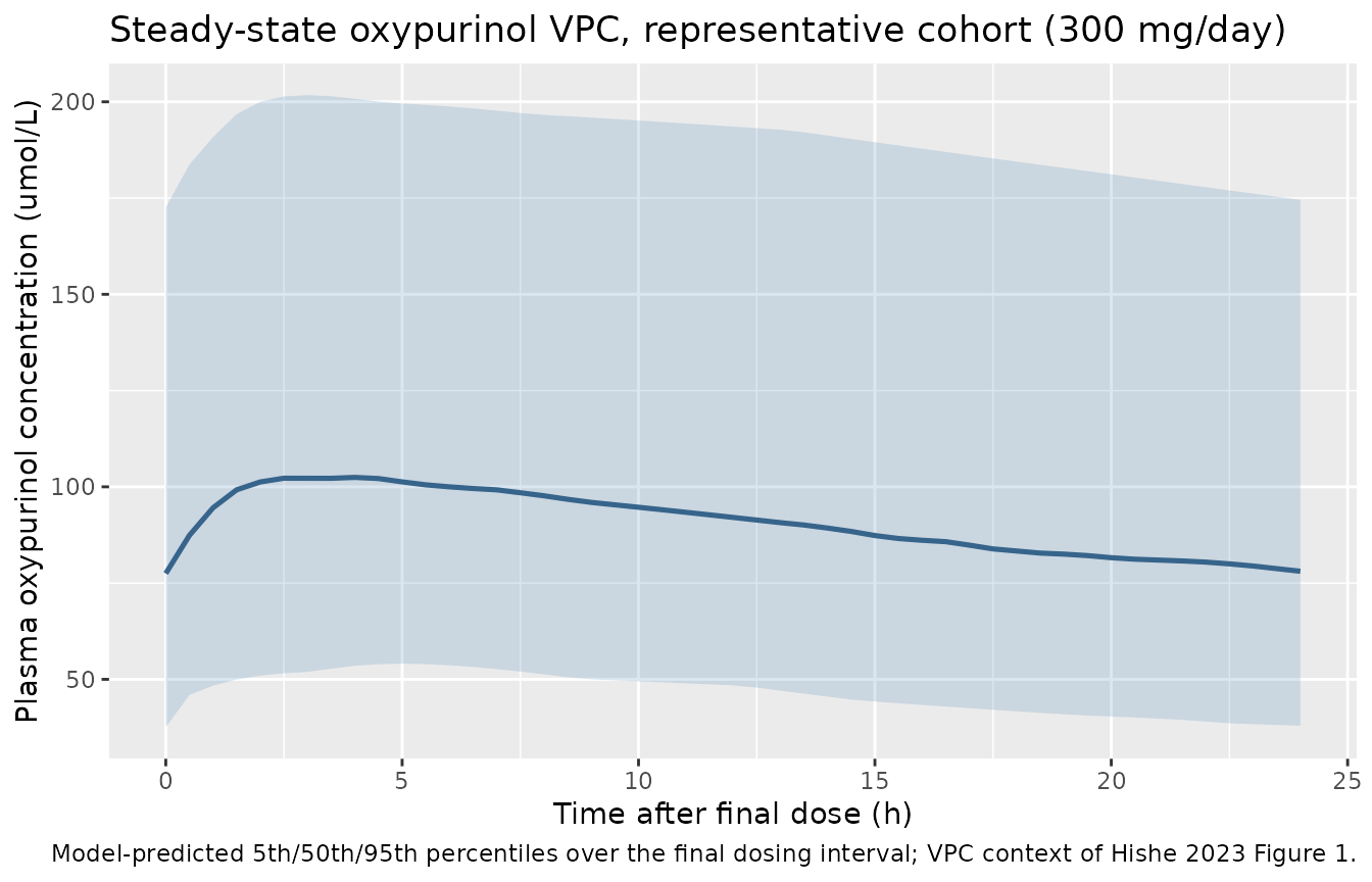
Clearance covariate effects (Hishe 2023 Table 2)
The typical-value (random-effects-zeroed) individual clearance recovered for each covariate contrast reproduces the Table 2 multipliers exactly: diuretic 0.79, Pacific 1.25, and the renal / weight power terms.
cl_B <- sim_B |>
  group_by(stratum) |>
  summarise(cl = dplyr::first(cl), .groups = "drop")
ref_cl <- cl_B$cl[cl_B$stratum == "reference"]

cov_tab <- cl_B |>
  mutate(ratio_vs_ref = cl / ref_cl,
         expected = dplyr::case_when(
           stratum == "reference"  ~ 1,
           stratum == "+diuretic"  ~ 0.79,
           stratum == "+Pacific"   ~ 1.25,
           stratum == "CRCL 3 L/h" ~ (3 / 6)^0.58,
           stratum == "WT 100 kg"  ~ (100 / 70)^0.34
         ))

knitr::kable(
  cov_tab |>
    dplyr::rename("Stratum" = stratum, "CL (L/h)" = cl,
                  "Ratio vs reference" = ratio_vs_ref,
                  "Expected (Table 2)" = expected),
  digits = 4,
  caption = "Typical-value CL by covariate contrast vs the Hishe 2023 Table 2 multipliers."
)| Stratum | CL (L/h) | Ratio vs reference | Expected (Table 2) |
|---|---|---|---|
| +Pacific | 1.2125 | 1.2500 | 1.2500 |
| +diuretic | 0.7663 | 0.7900 | 0.7900 |
| CRCL 3 L/h | 0.6489 | 0.6690 | 0.6690 |
| WT 100 kg | 1.0951 | 1.1289 | 1.1289 |
| reference | 0.9700 | 1.0000 | 1.0000 |
PKNCA validation
PKNCA is run on the representative cohort over the final 24-h steady-state dosing interval, re-anchored to time = 0. Dose / AUC0-tau recovers the apparent oxypurinol clearance CL/F, which is compared against the Hishe 2023 typical-value thetaCL = 0.97 L/h after accounting for the cohort covariate distribution.
last_dose_time <- (n_doses - 1L) * tau
nca_conc <- sim_A_num |>
  dplyr::filter(time >= last_dose_time, time <= last_dose_time + tau) |>
  dplyr::mutate(time = time - last_dose_time) |>
  dplyr::select(id, time, Cc) |>
  dplyr::filter(!is.na(Cc))

# Time-zero anchor: the observation grid starts exactly at the final dose, so
# every subject already has a t = 0 row (the steady-state trough, not zero).
stopifnot(all(tapply(nca_conc$time, nca_conc$id, min) == 0))

# Oxypurinol-equivalent dose in umol, so dose / AUC (umol/L) gives CL in L/h.
dose_umol <- 0.9 * dose_mg / 136.11 * 1000
nca_dose <- nca_conc |>
  dplyr::distinct(id) |>
  dplyr::mutate(time = 0, amt = dose_umol)

conc_obj <- PKNCA::PKNCAconc(nca_conc, Cc ~ time | id, concu = "umol/L", timeu = "hr")
dose_obj <- PKNCA::PKNCAdose(nca_dose, amt ~ time | id, doseu = "umol")

intervals_ss <- data.frame(
  start = 0, end = tau,
  cmax = TRUE, tmax = TRUE, cmin = TRUE, cav = TRUE, auclast = TRUE
)
nca_ss <- PKNCA::pk.nca(PKNCA::PKNCAdata(conc_obj, dose_obj, intervals = intervals_ss))
knitr::kable(
  summary(nca_ss),
  caption = paste("Steady-state NCA over the final 24-h interval,",
                  "representative cohort (full BSV + residual error).")
)| Interval Start | Interval End | N | AUClast (hr*umol/L) | Cmax (umol/L) | Cmin (umol/L) | Tmax (hr) | Cav (umol/L) |
|---|---|---|---|---|---|---|---|
| 0 | 24 | 200 | 2240 [43.9] | 104 [42.0] | 79.9 [47.9] | 3.50 [0.500, 9.50] | 93.4 [43.9] |
Comparison against the published model
Hishe 2023 does not report a non-compartmental Cmax / AUC table, so the validation compares the recovered apparent clearance and the cohort steady-state exposure against the published structural quantities: thetaCL = 0.97 L/h (typical patient at the reference covariate state) and the observed median plasma oxypurinol of 112 umol/L (Table S4).
nca_df <- as.data.frame(nca_ss$result)
auc_per_id <- nca_df |>
  dplyr::filter(PPTESTCD == "auclast") |>
  dplyr::transmute(id, auc_tau = PPORRES)
cl_per_id <- auc_per_id |>
  dplyr::mutate(cl_recovered = dose_umol / auc_tau)

# Typical-value CL/F at the reference covariate state, from the deterministic
# contrast simulation (thetaCL with all covariates at reference = 0.97 L/h).
cl_ref_typ <- cl_B$cl[cl_B$stratum == "reference"]

# Cohort median steady-state oxypurinol concentration.
cohort_med_css <- median(sim_A_num$Cc[sim_A_num$time >= last_dose_time], na.rm = TRUE)

summary_tab <- tibble::tibble(
  Quantity = c("Typical CL/F at reference covariates (L/h)",
               "Cohort median steady-state Cc (umol/L)"),
  Simulated = c(round(cl_ref_typ, 3), round(cohort_med_css, 1)),
  Published = c(0.97, 112)
)
knitr::kable(summary_tab, caption = "Simulated vs Hishe 2023 published quantities.")| Quantity | Simulated | Published |
|---|---|---|
| Typical CL/F at reference covariates (L/h) | 0.97 | 0.97 |
| Cohort median steady-state Cc (umol/L) | 91.10 | 112.00 |
# Structural checks.
# (1) The typical CL/F at the reference covariate state IS thetaCL by
#     construction, so it must equal 0.97 L/h to numerical tolerance.
stopifnot(abs(cl_ref_typ - 0.97) < 1e-3)

# (2) The cohort-level CL recovered by NCA (median) should track the covariate-
#     weighted typical CL. A mis-transcribed CL, dose or unit would move the
#     whole distribution by tens of percent; the bound is generous enough to be
#     robust to which subjects land in the tails but tight enough to catch a
#     structural error.
#     Observed across renders: about 0.9 L/h.
med_cl_recovered <- median(cl_per_id$cl_recovered, na.rm = TRUE)
stopifnot(med_cl_recovered > 0.65, med_cl_recovered < 1.25)

# (3) The cohort steady-state exposure should bracket the observed median
#     (112 umol/L) within a physiologically plausible envelope. This is a
#     different quantity (median of sampled concentrations across a mixed
#     cohort vs the paper's observed median), so a wide structural bound is
#     used rather than a tight one. Observed across renders: about 90 umol/L.
stopifnot(cohort_med_css > 60, cohort_med_css < 160)
The typical CL/F at the reference covariate state equals thetaCL by construction. The representative cohort’s median steady-state oxypurinol concentration (about 90 umol/L at 300 mg/day) sits below the observed median of 112 umol/L in Table S4. The observed median pools samples across doses of 50-900 mg/day, real sampling times and correlated covariates (lower doses are given in renal impairment), none of which the virtual cohort reproduces, so it is only an approximate anchor; see the Assumptions for how it bears on the dose conversion.
Assumptions and deviations
-
Allopurinol-to-oxypurinol conversion (molar
reading). Only oxypurinol was measured; the paper relates the
allopurinol dose to oxypurinol with a 0.9 conversion factor (Hishe 2023
Appendix S1, citing Day 2007). The packaged model applies this as a
molar conversion: 0.9 of the allopurinol molecules
become oxypurinol (1:1 molar), so
Cc = 0.9 * central / vc * 1000 / 136.11(umol/L), using the allopurinol molecular weight 136.11 g/mol. This is the physically correct reading of a conversion fraction, matches the same research group’s parent-metabolite convention (Wright_2013_allopurinol.R), and is the closer of the two readings to the observed data: the representative cohort’s median steady-state concentration is about 90 umol/L under the molar reading and about 80 umol/L under the mass reading, against the observed median of 112 umol/L (Table S4). The maintainers considered a mass reading (0.9 * mg allopurinol taken as mg oxypurinol, then divided by the oxypurinol molecular weight 152.11), which is how the cited origin of the 0.9 factor (Day 2007) and the siblingStocker_2012_oxypurinol.Rexpress the relationship; that reading predicts concentrations about 12% lower (the molecular-weight ratio 152.11/136.11). The paper does not state which molecular weight turned the allopurinol dose into the NONMEM oxypurinol amount, so the 12% band is a genuine ambiguity; the molar reading was chosen on the closer agreement with the observed median and the within-group precedent. - Between-subject variability reported as log-scale SD. Hishe 2023 Table 2 reports omega as “CV%”. The Appendix S2 control stream fixes the Ka variance at omega^2 = 0.388, and sqrt(0.388) = 0.623 = the reported 62.3% CV, confirming that the printed “CV%” is the log-scale standard deviation expressed as a percentage (the NONMEM-tradition CV ~= omega). The packaged model therefore encodes omega^2 = (CV%/100)^2 for CL (29.8%), V (41.3%) and Ka (62.3%), with the CL/V covariance from the reported correlation 0.41.
-
Per-study residual error and the reference study. A
separate combined additive + proportional residual error was estimated
for each of the five pooled studies (Table 2). The packaged model
selects the per-study error via the
STUDY_STAMP2011/STUDY_STAMP2012/STUDY_STAMP2013/STUDY_WRIGHT2016indicator columns; when all four are 0 the error defaults to Study 5 (Stamp 2017), the largest sub-cohort (176 of 300). This vignette leaves all four at 0, so the VPC and NCA use the Study-5 residual. -
Creatinine clearance units.
CRCLis Cockcroft-Gault creatinine clearance standardised to 70 kg and expressed in L/h (normalisation standard 6 L/h = 100 mL/min/70 kg), matching the siblingWright_2016_allopurinol.R. The virtual cohort drawsCRCLin L/h (cohort median 3.78 L/h = 63 mL/min). -
Volume weight exponent fixed. The Results equation
writes
V/F = thetaV * (WT/70)with no exponent reported in Table 2, so the weight exponent on volume is held fixed at the theoretical value 1.0 (linear). -
Urate-transporter genotypes not modelled. Seven
SNPs (ABCG2 rs2231142 and rs10011796, SLC2A9 rs11942223, SLC17A1
rs1183201, SLC22A12 rs3825018, SLC22A11 rs17300741, ABCC4 rs4148500)
were screened. ABCG2 rs2231142 (+24%) and SLC17A1 rs1183201 (+22%) were
significant univariately but not retained in the multivariate model,
where they were confounded by correlated creatinine clearance, weight,
age, diuretic use and ethnicity. The packaged model has no SNP
covariates; the screened variants are recorded in the model file’s
covariatesDataExcludedmetadata. - Virtual-cohort distributions. The covariate distributions are log-normal approximations to the Hishe 2023 Table S4 marginals (weight, creatinine clearance) with independent 37% diuretic and 21% Pacific prevalences; the original per-subject covariate data are not public, so inter-covariate correlations (e.g. the reported association of the ABCG2 T allele with higher CrCl, lower diuretic use and Pacific ethnicity) are not reproduced.
- Errata. No erratum or corrigendum to Hishe 2023 was found in the sources on hand as of this writing (2026-10); the maintainers should reconfirm against the Clinical and Translational Science corrections feed if a re-extraction is undertaken.