Vancomycin in pediatric liver transplant recipients (Shoji 2021)
Source:vignettes/articles/Shoji_2021_vancomycin.Rmd
Shoji_2021_vancomycin.RmdModel and source
- Citation: Shoji K, Saito J, Nakagawa H, Funaki T, Fukuda A, Sakamoto S, Kasahara M, Momper JD, Capparelli EV, Miyairi I. Population pharmacokinetics and dosing optimization of vancomycin in pediatric liver transplant recipients. Microbiol Spectr. 2021;9(2):e00460-21. doi:10.1128/Spectrum.00460-21
- Description: One-compartment IV population PK model for vancomycin in pediatric liver transplant recipients aged 1-186 months (Shoji 2021), developed from 1,158 routine therapeutic-drug-monitoring concentrations in 161 children (270 treatment episodes) at a single Japanese pediatric transplant center. Clearance scales with body weight to the fixed 0.75 power and with power functions of serum creatinine (reference 0.16 mg/dL, exponent -0.70) and days from liver transplantation to the start of vancomycin (reference 17 days, exponent -0.09), so clearance is highest early after transplant and at low serum creatinine; volume of distribution is proportional to body weight. The final-model between-subject and residual variances are not reported (Table 3 prints them for the base model only) and are encoded as zero.
- Article: https://doi.org/10.1128/Spectrum.00460-21 (open access, PMC8510181)
- Supplement (Fig. S1 goodness-of-fit plots, Table S1 dosing
simulations by creatinine clearance):
spectrum00460-21_supp_1_seq2.pdf, published with the open-access article (PMC8510181).
Shoji 2021 is a single-center retrospective population-PK analysis of intravenous vancomycin in children after liver transplantation, followed by Monte Carlo dosing simulations. The final model is a one-compartment model with allometric body-weight scaling, and with serum creatinine and the number of days from liver transplantation to the start of vancomycin (DFLT) as power-function covariates on clearance.
Population
161 pediatric liver transplant recipients (270 vancomycin treatment episodes, 1,158 serum concentrations) treated at the National Center for Child Health and Development, Tokyo, between 2006 and 2014 (Shoji 2021 Table 1). Median age 13.3 months (IQR 7.6-53.5, range 1-186 months); median weight 9.1 kg (IQR 6.8-16.2, range 3.1-61.0); 55.3% female. Underlying diseases: biliary atresia 52.2%, metabolic disease 18.6%, fulminant hepatitis 16.1%, liver cirrhosis and liver fibrosis 4.3% each, vascular abnormalities 2.5%, liver tumor 1.9%. Median serum creatinine 0.16 mg/dL (IQR 0.12-0.23, range 0.06-5.43); median DFLT 17 days (IQR 6-31, range 0-357). All patients received tacrolimus (median trough 8.2 ug/mL). Patients on renal replacement therapy were excluded. The median dose was 15.0 mg/kg (IQR 14.0-15.0), usually every 6 h (ages 1 month to 12 years) or every 8 h (13-17 years).
The same information is available programmatically via
readModelDb("Shoji_2021_vancomycin")()$population.
Source trace
Each ini() entry in
inst/modeldb/specificDrugs/Shoji_2021_vancomycin.R carries
an in-file comment giving its origin; the table collects them.
| Equation / parameter | Value | Source location |
|---|---|---|
lcl (theta_CL) |
0.29 L/h/kg^0.75 | Table 3 final model, RSE 4.13%; bootstrap median 0.29 (95% CI 0.26-0.32) |
lvc (theta_V) |
1.00 L/kg | Table 3 final model, RSE 5.97%; bootstrap median 1.00 (95% CI 0.89-1.14) |
e_creat_cl (theta_sCr) |
-0.70 | Table 3 final model, RSE 8.23%; bootstrap median -0.69 (95% CI -0.79 to -0.57) |
e_pod_cl (theta_DFLT) |
-0.09 | Table 3 final model, RSE 34.8%; bootstrap median -0.09 (95% CI -0.15 to -0.03) |
e_wt_cl |
0.75, fixed | Methods (“scaled allometrically by subject weight (weight^0.75)”); Table 3 footnote b |
e_wt_vc |
1, fixed | Methods (“scaled by subject weight (weight^1.0)”); Table 3 footnote c |
etalcl, etalvc
|
0, fixed | Exponential IIV declared in the Results equations; final-model magnitudes not printed (see Errata) |
propSd, addSd
|
0, fixed | Results: “an additive/proportional error model was selected”; final-model magnitudes not printed (see Errata) |
d/dt(central) |
n/a | Results: “A one-compartment model was selected as the structural model” |
cl <- ... |
n/a | Results:
TVCL(l/h) = CLpop x (sCr/0.16)^theta_sCr x (DFLT/17)^theta_DFLT x wt^0.75 x exp(eta_CL);
Table 3 footnote b |
vc <- ... |
n/a | Results: TVVi = Vpop x wt x exp(eta_V); Table 3
footnote c |
| Reference sCr 0.16 mg/dL, DFLT 17 days | n/a | Table 1 cohort medians |
The final-model equations are typeset as images in the article; the
forms above were read from the publisher’s equation image
spectrum.00460-21-m001.jpg, deposited with the article, and
match Table 3 footnote b.
Check 1 – typical values against the published post hoc averages
Shoji 2021 Results report post hoc average clearance and volume of
0.18 +/- 0.08 L/h/kg and 1.01 +/- 0.35 L/kg. At the cohort medians (9.1
kg, sCr 0.16 mg/dL, DFLT 17 days), the covariate terms for sCr and DFLT
are exactly 1, so the typical clearance per kg is
0.29 * 9.1^-0.25 and the typical volume per kg is exactly
theta_V.
mod <- readModelDb("Shoji_2021_vancomycin") |> rxode2::zeroRe()
#> ℹ parameter labels from comments will be replaced by 'label()'

typical_cl_per_kg <- 0.29 * 9.1^0.75 / 9.1
typical_v_per_kg <- 1.00

# Solve the packaged model at the medians and read back its own cl and vc.
ev_med <- data.frame(
  id = 1L, time = c(0, 1), amt = c(15 * 9.1, 0), rate = c(15 * 9.1, 0),
  evid = c(1L, 0L), cmt = "central", WT = 9.1, CREAT = 0.16, POD = 17
)
sim_med <- rxode2::rxSolve(mod, events = ev_med) |> as.data.frame()
#> ℹ omega/sigma items treated as zero: 'etalcl', 'etalvc'

stopifnot(
  abs(sim_med$cl[1] / 9.1 - typical_cl_per_kg) < 1e-10,
  abs(sim_med$vc[1] / 9.1 - typical_v_per_kg) < 1e-10,
  # The typical clearance of a median child sits within one post hoc SD of the
  # published post hoc average (0.18 +/- 0.08 L/h/kg) ...
  abs(typical_cl_per_kg - 0.18) < 0.08,
  # ... and the typical volume is within 0.01 L/kg of it (1.01 +/- 0.35 L/kg).
  abs(typical_v_per_kg - 1.01) < 0.02
)

tibble(
  Quantity = c("CL (L/h/kg)", "V (L/kg)"),
  `Model, median child` = signif(c(typical_cl_per_kg, typical_v_per_kg), 3),
  `Shoji 2021 post hoc mean (SD)` = c("0.18 (0.08)", "1.01 (0.35)")
) |>
knitr::kable()| Quantity | Model, median child | Shoji 2021 post hoc mean (SD) |
|---|---|---|
| CL (L/h/kg) | 0.167 | 0.18 (0.08) |
| V (L/kg) | 1.000 | 1.01 (0.35) |
Replicating Figure 1 – clearance against serum creatinine by DFLT
Figure 1 of Shoji 2021 plots post hoc clearance (L/h/kg) against serum creatinine on a log axis, separately for episodes with DFLT < 14 days and >= 14 days. Without the individual random effects the model gives the typical curves below, drawn for a 9.1 kg child at DFLT 7 days and 30 days (roughly the centres of the two groups). The published scatter spans about 0.02-0.42 L/h/kg and falls steeply between sCr 0.1 and 0.5 mg/dL, the shape of a power function with exponent -0.70.
fig1 <- expand.grid(
  CREAT = exp(seq(log(0.05), log(5), length.out = 200)),
  POD = c(7, 30)
) |>
  mutate(
    cl_per_kg = 0.29 * 9.1^0.75 * (CREAT / 0.16)^-0.70 * (POD / 17)^-0.09 / 9.1,
    group = ifelse(POD < 14, "DFLT < 14 days (7 days shown)", "DFLT >= 14 days (30 days shown)")
  )

# The DFLT effect: going from day 7 to day 30 lowers clearance by a fixed factor
# at every creatinine value.
pod_ratio <- (7 / 17)^-0.09 / (30 / 17)^-0.09
stopifnot(abs(pod_ratio - (30 / 7)^0.09) < 1e-12)
pod_ratio
#> [1] 1.13994

ggplot(fig1, aes(CREAT, cl_per_kg, linetype = group)) +
  geom_line() +
  scale_x_log10(breaks = c(0.05, 0.5, 5)) +
  coord_cartesian(ylim = c(0, 0.5)) +
  labs(x = "Serum creatinine (mg/dL)", y = "Vancomycin clearance (L/h/kg)", linetype = NULL) +
  theme_bw() +
  theme(legend.position = "bottom")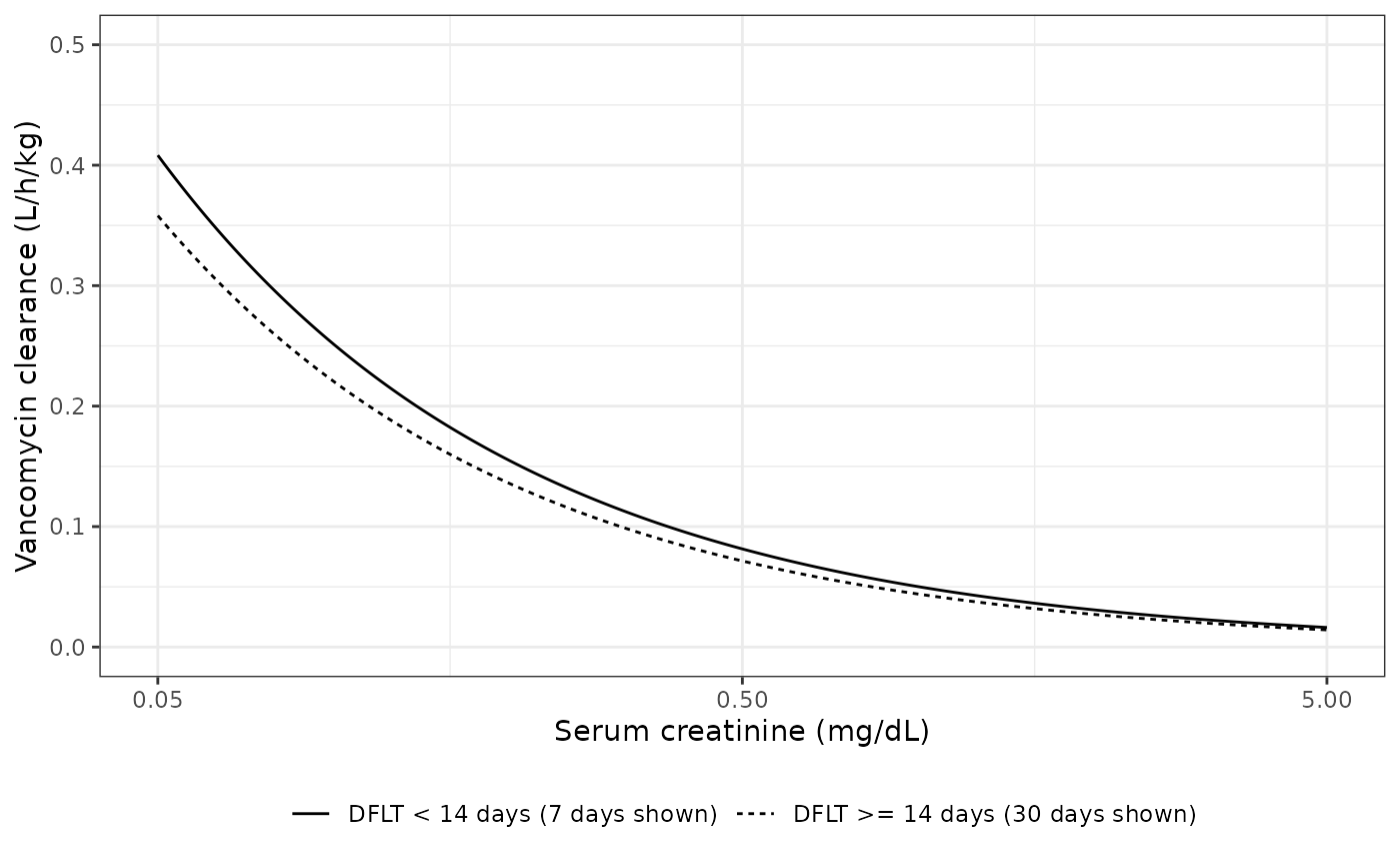
Typical clearance against serum creatinine for a 9.1 kg child. Replicates the shape of Figure 1 of Shoji 2021 (which plots post hoc estimates).
The two curves differ by only 14%, which is all a DFLT exponent of -0.09 can produce between day 7 and day 30. The published figure separates the groups more than that, because the post hoc estimates also carry the random effects and the creatinine values differ between the groups.
Virtual cohort
The article does not publish its individual data. The cohort below is built from the Table 1 medians and interquartile ranges, each covariate taken as log-normal (median = the published median, log-scale SD from the published IQR) and truncated to the published range. Because the packaged model has no between-subject variability, a simulation is a deterministic function of the covariates, so the cohort is a fixed quantile grid rather than a random draw and every number below is reproducible on any machine. DFLT is truncated below at 1 day, because the covariate term is infinite at 0 (see Errata). The covariates are taken as independent; the article does not report their correlations.
n_per_arm <- 100L
u <- ppoints(n_per_arm)
i <- seq_len(n_per_arm)
shift <- function(k) ((i + k - 1L) %% n_per_arm) + 1L

# Truncated log-normal quantile: median m, IQR (q1, q3), range (lo, hi).
qtrunc_lnorm <- function(p, m, q1, q3, lo, hi) {
  sdlog <- log(q3 / q1) / (2 * qnorm(0.75))
  plo <- plnorm(lo, log(m), sdlog)
  phi <- plnorm(hi, log(m), sdlog)
  qlnorm(plo + p * (phi - plo), log(m), sdlog)
}

covariates <- tibble(
  cohort_id = i,
  WT = qtrunc_lnorm(u, 9.1, 6.8, 16.2, 3.1, 61.0), # Table 1 wt, kg
  CREAT = qtrunc_lnorm(u[shift(33L)], 0.16, 0.12, 0.23, 0.06, 5.43), # Table 1 sCr, mg/dL
  POD = qtrunc_lnorm(u[shift(66L)], 17, 6, 31, 1, 357) # Table 1 DFLT, days
)

stopifnot(
  abs(median(covariates$WT) - 9.1) / 9.1 < 0.1,
  abs(median(covariates$CREAT) - 0.16) / 0.16 < 0.1,
  abs(median(covariates$POD) - 17) / 17 < 0.1,
  min(covariates$POD) >= 1
)

summary(covariates[, c("WT", "CREAT", "POD")])
#>        WT             CREAT              POD
#>  Min.   : 3.194   Min.   :0.06262   Min.   :  1.207
#>  1st Qu.: 6.342   1st Qu.:0.11874   1st Qu.:  7.722
#>  Median : 9.441   Median :0.16205   Median : 17.100
#>  Mean   :11.507   Mean   :0.18215   Mean   : 32.545
#>  3rd Qu.:14.285   3rd Qu.:0.22247   3rd Qu.: 37.976
#>  Max.   :45.301   Max.   :0.55612   Max.   :274.986
Simulation
The three regimens of Shoji 2021 Table 4 are simulated for 7 days as 1-hour infusions, which is long enough to reach steady state in every cohort member. The article does not state the infusion duration; 1 hour is an assumption.
regimens <- tibble(
  regimen = c("15 mg/kg q8h", "15 mg/kg q6h", "20 mg/kg q6h"),
  dose_mgkg = c(15, 15, 20),
  tau = c(8, 6, 6)
)

make_arm <- function(k) {
  r <- regimens[k, ]
  dose_times <- seq(0, 168 - r$tau, by = r$tau)
  obs_times <- sort(unique(c(seq(144, 168, by = 0.05))))
  cov_k <- covariates |> mutate(id = cohort_id + (k - 1L) * n_per_arm)
  doses <- tidyr::crossing(cov_k, time = dose_times) |>
    mutate(amt = r$dose_mgkg * WT, rate = amt / 1, evid = 1L)
  obs <- tidyr::crossing(cov_k, time = obs_times) |>
    mutate(amt = 0, rate = 0, evid = 0L)
  bind_rows(doses, obs) |>
    mutate(cmt = "central", regimen = r$regimen, tau = r$tau) |>
    arrange(id, time, desc(evid))
}
events <- bind_rows(lapply(seq_len(nrow(regimens)), make_arm))

sim <- rxode2::rxSolve(
  mod,
  events = as.data.frame(events),
  keep = c("regimen", "tau", "WT", "CREAT", "POD")
) |>
  as.data.frame()
#> ℹ omega/sigma items treated as zero: 'etalcl', 'etalvc'
#> Warning: multi-subject simulation without without 'omega'

stopifnot(
  length(unique(sim$id)) == 3L * n_per_arm,
  all(is.finite(sim$Cc)),
  all(sim$Cc > 0)
)
Typical steady-state profiles
The median child’s steady-state profile over the last dosing interval of each regimen. Figure 2 of Shoji 2021 (the VPC, which pools every dose level and dosing interval against time after dose) has a simulated median of about 18 ug/mL just after the dose, falling to about 10 ug/mL by 5 h and about 5 ug/mL by 10 h. The typical peaks and troughs, tabulated below the figure, lie inside that band.
ev_typ <- bind_rows(lapply(seq_len(nrow(regimens)), function(k) {
  r <- regimens[k, ]
  bind_rows(
    tibble(time = seq(0, 168 - r$tau, by = r$tau), amt = r$dose_mgkg * 9.1, evid = 1L),
    tibble(time = seq(168 - r$tau, 168, by = 0.05), amt = 0, evid = 0L)
  ) |>
    mutate(id = k, rate = amt, cmt = "central", WT = 9.1, CREAT = 0.16, POD = 17, regimen = r$regimen)
}))
sim_typ <- rxode2::rxSolve(mod, events = as.data.frame(ev_typ), keep = "regimen") |>
  as.data.frame() |>
  group_by(regimen) |>
  mutate(tad = time - min(time)) |>
  ungroup()
#> ℹ omega/sigma items treated as zero: 'etalcl', 'etalvc'
#> Warning: multi-subject simulation without without 'omega'

ggplot(sim_typ, aes(tad, Cc, colour = regimen)) +
  geom_line() +
  labs(x = "Time after dose (h)", y = "Vancomycin (ug/mL)", colour = NULL) +
  theme_bw() +
  theme(legend.position = "bottom")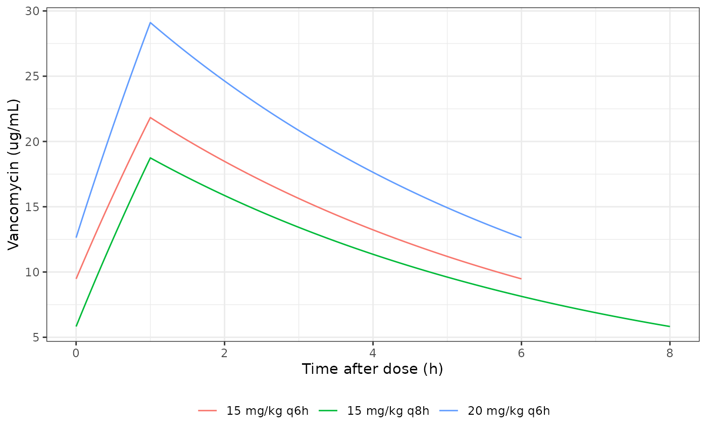
Typical steady-state concentration-time profiles for a 9.1 kg child with sCr 0.16 mg/dL and DFLT 17 days.
typ_peak_trough <- sim_typ |>
  group_by(regimen) |>
  summarise(peak = max(Cc), trough = Cc[which.max(tad)], .groups = "drop")

# Typical peaks and troughs within the 5-35 ug/mL span of the Figure 2 median.
stopifnot(
  all(typ_peak_trough$peak > 15 & typ_peak_trough$peak < 35),
  all(typ_peak_trough$trough > 4 & typ_peak_trough$trough < 15)
)

typ_peak_trough |>
  dplyr::rename(Regimen = regimen, `Peak (ug/mL)` = peak, `Trough (ug/mL)` = trough) |>
knitr::kable(digits = 1)| Regimen | Peak (ug/mL) | Trough (ug/mL) |
|---|---|---|
| 15 mg/kg q6h | 21.8 | 9.5 |
| 15 mg/kg q8h | 18.7 | 5.8 |
| 20 mg/kg q6h | 29.1 | 12.6 |
PKNCA – steady-state AUC over 24 h
PKNCA computes each subject’s AUC over the final 24 h (144-168 h) and the trough at 168 h. For a linear one-compartment model at steady state, AUC over a 24-h window is exactly the daily dose divided by clearance. Both sides use the same parameters, so the difference is only the numerical error of the trapezoidal rule and a tight bound is the right gate.
sim_nca <- sim |>
  dplyr::filter(!is.na(Cc)) |>
  dplyr::select(id, time, Cc, regimen)

conc_obj <- PKNCA::PKNCAconc(
  as.data.frame(sim_nca), Cc ~ time | regimen + id,
  concu = "ug/mL", timeu = "h"
)
dose_df <- events |>
  dplyr::filter(evid == 1L) |>
  dplyr::select(id, time, amt, regimen)
dose_obj <- PKNCA::PKNCAdose(
  as.data.frame(dose_df), amt ~ time | regimen + id,
  doseu = "mg"
)
intervals <- data.frame(start = 144, end = 168, auclast = TRUE, cmax = TRUE, clast.obs = TRUE)

nca_res <- PKNCA::pk.nca(PKNCA::PKNCAdata(conc_obj, dose_obj, intervals = intervals))

nca_wide <- as.data.frame(nca_res) |>
  dplyr::select(regimen, id, PPTESTCD, PPORRES) |>
  tidyr::pivot_wider(names_from = PPTESTCD, values_from = PPORRES)

per_subject <- sim |>
  group_by(id) |>
  slice(1) |>
  ungroup() |>
  select(id, cl, WT, CREAT, POD) |>
  left_join(events |> distinct(id, regimen, tau), by = "id") |>
  left_join(regimens |> select(regimen, dose_mgkg), by = "regimen")

auc_chk <- nca_wide |>
  left_join(per_subject, by = c("id", "regimen")) |>
  mutate(
    auc24_closed = dose_mgkg * WT * 24 / tau / cl,
    auc_relerr = abs(auclast - auc24_closed) / auc24_closed
  )

stopifnot(
  nrow(auc_chk) == 3L * n_per_arm,
  all(is.finite(auc_chk$auc_relerr)),
  max(auc_chk$auc_relerr) < 0.005
)
max(auc_chk$auc_relerr)
#> [1] 2.144767e-05
Comparison with Table 4 – target attainment by regimen
Shoji 2021 Table 4 reports the percentage of 1,000 simulated patients reaching a trough above 10 ug/mL and an AUC24/MIC of at least 400. Those percentages depend on the between-subject variability and on the covariate joint distribution of the authors’ simulation, neither of which is reproducible here. What the packaged model does determine is the typical (median-covariate) child, and a regimen should reach a target for the typical child exactly when more than half of the published population reaches it. That is checked below for the AUC24/MIC target, which the typical child clears or misses by at least 10% in every row.
typ_auc24 <- regimens |>
  mutate(
    cl_typ = 0.29 * 9.1^0.75,
    auc24 = dose_mgkg * 9.1 * 24 / tau / cl_typ,
    # Shoji 2021 Table 4, 'Total' column.
    pub_auc_mic05 = c(100.0, 100.0, 100.0),
    pub_auc_mic1 = c(7.4, 16.3, 88.1)
  )

stopifnot(
  # MIC 0.5: every regimen reaches AUC24 >= 200 for the typical child (Table 4: 100%).
  all(typ_auc24$auc24 >= 200),
  # MIC 1: the typical child reaches AUC24 >= 400 exactly where Table 4 exceeds 50%.
  identical(typ_auc24$auc24 >= 400, typ_auc24$pub_auc_mic1 > 50)
)

# Cohort attainment (covariate spread only, no between-subject variability).
cohort_pta <- auc_chk |>
  group_by(regimen) |>
  summarise(
    auc_mic05 = 100 * mean(auclast / 0.5 >= 400),
    auc_mic1 = 100 * mean(auclast / 1 >= 400),
    trough10 = 100 * mean(clast.obs > 10),
    .groups = "drop"
  )

typ_auc24 |>
  left_join(cohort_pta, by = "regimen") |>
  mutate(
    pub_trough10 = c(31.2, 54.0, 71.6),
    auc24 = round(auc24)
  ) |>
  select(regimen, auc24, pub_auc_mic1, auc_mic1, pub_auc_mic05, auc_mic05, pub_trough10, trough10) |>
  dplyr::rename(
    Regimen = regimen,
    `Typical AUC24 (ug*h/mL)` = auc24,
    `AUC24/MIC>=400, MIC 1: Table 4 (%)` = pub_auc_mic1,
    `AUC24/MIC>=400, MIC 1: cohort (%)` = auc_mic1,
    `AUC24/MIC>=400, MIC 0.5: Table 4 (%)` = pub_auc_mic05,
    `AUC24/MIC>=400, MIC 0.5: cohort (%)` = auc_mic05,
    `Trough>10: Table 4 (%)` = pub_trough10,
    `Trough>10: cohort (%)` = trough10
  ) |>
knitr::kable(digits = 1)| Regimen | Typical AUC24 (ug*h/mL) | AUC24/MIC>=400, MIC 1: Table 4 (%) | AUC24/MIC>=400, MIC 1: cohort (%) | AUC24/MIC>=400, MIC 0.5: Table 4 (%) | AUC24/MIC>=400, MIC 0.5: cohort (%) | Trough>10: Table 4 (%) | Trough>10: cohort (%) |
|---|---|---|---|---|---|---|---|
| 15 mg/kg q8h | 270 | 7.4 | 10 | 100 | 88 | 31.2 | 13 |
| 15 mg/kg q6h | 359 | 16.3 | 38 | 100 | 99 | 54.0 | 48 |
| 20 mg/kg q6h | 479 | 88.1 | 77 | 100 | 100 | 71.6 | 74 |
The cohort percentages come from covariate spread alone and are shown for orientation only; they are not expected to match the published values.
Assumptions and deviations
-
Between-subject and residual variability are zero.
Shoji 2021 Table 3 prints
% omega CL= 46.47 (RSE 2.88%),% omega Vc= 48.14 (RSE 6.55%) and a proportional residual error of 56.5% (RSE 4.02%) only in the base-model column; the final-model and bootstrap columns are blank for these rows. The base model has no serum-creatinine term, and serum creatinine alone lowered the objective function by 435 points (Table 2), so the base-model clearance variability overstates the final model’s. Combining final-model fixed effects with base-model variances would give a model the authors never fitted, so the final-model variances are encoded asfixed(0). Users who need stochastic simulations can supply their own values; the base-model values above are upper-bound guides for clearance and plausible guides for volume. Final-model eta shrinkage was 22.0% (CL) and 27.0% (V), and epsilon shrinkage 4.55%. -
Residual error form. The Results state that “an
additive/proportional error model was selected”, but Table 3 prints only
a proportional term (for the base model). The model carries both
propSdandaddSd, each fixed at 0. -
DFLT = 0. Table 1 reports DFLT from 0 days, but
with a negative exponent the printed term
(DFLT/17)^-0.09is infinite at 0. The article does not say how episodes starting on the day of transplant were coded. The model is encoded as printed and needsPOD > 0; this vignette usesPOD >= 1. -
DFLT is a per-episode constant. It is defined as
the days from transplantation to the first day of vancomycin,
and it is stored in the canonical
PODcolumn. Supply the value at the start of the treatment episode on every row, not a day count that advances with each observation. - Allometric weight enters unnormalised. theta_CL is per kg^0.75 and theta_V per kg, as in the published equations, not relative to a 70 kg reference.
- Infusion duration. Not stated in the article; 1 hour is used here.
- Virtual cohort. Log-normal covariates matched to the Table 1 medians and IQRs, truncated to the published ranges, and taken as independent.
Errata noted in the source
- Table 3 footnote c prints
V (l) = theta_V x wt x exp(eta_CL); the Results equation hasexp(eta_V), which is used here. - The Results text says “only 16% of the patients with a DFLT of <14 days achieved an AUC24/MIC of >=400 for an MIC of 1 ug/ml with … 15 mg/kg q6h”, but Table 4 gives 3.3% for DFLT < 14 days and 16.3% for the total population (the Abstract’s “16%” refers to all patients).
- Table 4, 20 mg/kg q6h, trough > 10 ug/mL: the total (71.6%) is lower than both subgroups (76.3% and 100.0%), which cannot happen for a weighted average of them. At least one of the three cells is misprinted.