Model and source
ui <- rxode2::rxode(readModelDb("May_2025_potravitug"))- Citation: May M, Bialek-Waldmann JK, Wright A, Gruver S, Grant J, Eicher B, Seidenberg J, Parzmair GP, Beck J. First-In-Human, Randomized, Placebo-Controlled, SAD and MAD Trial to Evaluate Safety, Tolerability, and PK/PD Modeling of Potravitug in Healthy Adults. Clin Transl Sci. 2025;18(8):e70316. doi:10.1111/cts.70316. Model parameters from Appendix S1 Table S1.
- Description: QSP. Semi-mechanistic PK/PD model of potravitug, a fully human IgG1 against the BK polyomavirus (BKPyV) major capsid protein VP1, in healthy adults (May 2025). Three drug compartments (central blood, peripheral tissues, kidney interstitial space) with first-order catabolism in every compartment and Pdist/Tdist inter-compartmental exchange; VP1 (BKPyV titer x 360 VP1 per virion) turns over in blood and kidney interstitial space and binds potravitug 1:1, the complex being cleared at the VP1 rate. Deterministic typical-subject (70 kg) model calibrated on cohort-mean SAD data; no IIV or residual error.
- Article: https://doi.org/10.1111/cts.70316 (open access; PMC12338083)
Potravitug is a fully human IgG1 antibody against VP1, the major capsid protein of BK polyomavirus (BKPyV), developed to treat BKPyV-DNAemia and BKPyV-associated nephropathy after kidney transplantation. May et al. (2025) report the first-in-human single and multiple ascending dose (SAD / MAD) trial and a semi-mechanistic PK/PD model, built in the Applied BioMath QSP Notebook, that was used to choose a 1000 mg IV dose given four times every four weeks.
The model (paper Figure 2) has three potravitug compartments –
central (blood), peripheral (other tissues) and the kidney interstitial
space (KIS), where BKPyV replicates. Potravitug is catabolised
first-order in every compartment and exchanges between blood and each
tissue under the Applied BioMath Pdist / Tdist
convention. VP1 (BKPyV titer x 360 VP1 copies per virion) is present in
blood and in the KIS, turns over with a 24 h half-life, and binds
potravitug 1:1; bound potravitug is cleared at the VP1 rate. Model
outputs are free potravitug in blood (Cc) and in the KIS
(Ckidney), both in ug/mL, and VP1 receptor occupancy (% of
total VP1 bound) in blood (ro_blood) and the KIS
(ro_kidney).
Population
The trial enrolled 40 healthy adults aged 18-50 years (BMI 18-32 kg/m^2) at a single Australian site (NCT05358106): 16 in the SAD part (12 active at 100, 500, 1000 or 2000 mg; 4 placebo) and 24 in the MAD part (18 active at 500, 1000 or 2000 mg every 4 weeks for 4 doses; 6 placebo). Half were female; 82.5% were White, 10% Asian, and one participant each was Black, Native Hawaiian or Other Pacific Islander, and Asian/White (paper Table 1). Body weight ranged 51.2-100.5 kg.
The PK/PD model was calibrated on the cohort-mean SAD serum concentrations for a typical 70 kg subject and validated against the MAD cohort means. It has no covariates, no between-subject variability and no residual error, so every simulation below is a single deterministic typical-subject profile per dose.
str(ui$population)
#> List of 11
#>  $ species       : chr "human"
#>  $ n_subjects    : int 40
#>  $ n_studies     : int 1
#>  $ age_range     : chr "18-50 years"
#>  $ weight_range  : chr "51.2-100.5 kg"
#>  $ sex_female_pct: num 50
#>  $ race_ethnicity: Named num [1:5] 82.5 10 2.5 2.5 2.5
#>   ..- attr(*, "names")= chr [1:5] "White" "Asian" "Black" "Pacific Islander" ...
#>  $ disease_state : chr "Healthy adult volunteers (BMI 18-32 kg/m^2); the VP1 sub-model represents an average BKPyV titer as in kidney-t"| __truncated__
#>  $ dose_range    : chr "Single IV infusion 100, 500, 1000 or 2000 mg (SAD, n = 12 active); 500, 1000 or 2000 mg IV every 4 weeks x 4 (M"| __truncated__
#>  $ regions       : chr "Australia (single centre, Adelaide)"
#>  $ notes         : chr "First-in-human trial NCT05358106; demographics from May 2025 Table 1 (40 randomized, of whom 30 received potrav"| __truncated__
Source trace
All parameter values are in Appendix S1 Table S1 of May 2025 (“PK/PD Modeling Parameters”); the model structure is from paper Figure 2, the PK/PD Modeling paragraphs of Methods and Results, and the “Model Assumptions” list under Table S1.
| Equation / parameter | Value | Source location |
|---|---|---|
lvc (central volume Vc) |
log(3.19 L) | Table S1, fit to PK data |
lvp (peripheral volume Vp) |
fixed log(13 L) | Table S1 (Shah and Betts 2012) |
lv_kidney (KIS volume) |
fixed log(0.005 L) | Table S1 (Shah and Betts 2012) |
lthalf_ab (potravitug half-life) |
log(31.4 day) | Table S1, fit to clinical data |
ltdist_ab (Tdist) |
log(52.4 h) | Table S1, fit to clinical data; unit inferred (see below) |
lpdist_ab (Pdist) |
log(0.441) | Table S1, fit to clinical data |
vp1_per_virion |
fixed 360 | Table S1 (Stehle 1996) |
titer_blood |
fixed 7e6 virions/L | Table S1 (Hariharan 2006) |
titer_kidney |
fixed 7e9 virions/L | Table S1 (Theodoropoulos 2013); 1000-fold blood, Model Assumptions |
lthalf_vp1 |
fixed log(1440 min) | Table S1 (Funk 2008); Model Assumptions
t_VP1_halflife = 24 hours
|
kon |
fixed 1e-3 1/nM/s | Table S1 (Schlosshauer 2004); Model Assumptions
kon = 0.001
|
kd |
fixed 60 pM | Table S1 (internal data); koff = Kd * kon, Model
Assumptions |
mw |
fixed 150000 g/mol | Not in the paper; typical IgG1 (see Assumptions) |
k_cp, k_pc, k_ck,
k_kc
|
derived | Table S1 Model Assumptions,
kij = ln(2)/Tdist_ij * Pdist_ij / (Pdist_ij + Vi/Vj),
kji = ln(2)/Tdist_ij / (1 + Pdist_ij * Vj/Vi)
|
kel in all compartments |
ln(2) / t1/2 | Figure 2 caption (“First order catabolic elimination of potravitug occurs in all compartments”) |
kdeg_vp1 |
ln(2) / 24 h | Model Assumptions
(k_VP1_el = ln(2)/t_VP1_halflife) |
| VP1 baselines | titer x 360 / N_A | Methods PK/PD Modeling (titers x VP1 per viral particle) |
| VP1 supply | zero-order, = baseline degradation | Model Assumptions (analytical solution holding KIS VP1 1000-fold above blood); see Assumptions |
| Complex elimination | kdeg_vp1 |
Model Assumptions (“When potravitug is bound to VP1, it is cleared at the rate of VP1”) |
| Binding | 1:1, kon * Ab * VP1 - koff * complex
|
Model Assumptions |
d/dt(central), d/dt(peripheral1),
d/dt(kidney)
|
– | Figure 2 and caption |
Baseline VP1 holds without drug
With no potravitug, VP1 must stay at its baseline in both compartments, and the kidney-to-blood concentration ratio must be the 1000-fold stated in the Model Assumptions.
ev_none <- rxode2::et(seq(0, 24 * 28, by = 24))
base <- as.data.frame(rxode2::rxSolve(ui, ev_none))
ini_vals <- setNames(ui$iniDf$est, ui$iniDf$name)
vc <- exp(ini_vals[["lvc"]])
v_kidney <- exp(ini_vals[["lv_kidney"]])
vp1_blood_nm <- base$target / vc
vp1_kidney_nm <- base$target_kidney / v_kidney
data.frame(
  quantity = c("VP1 in blood (fM)", "VP1 in KIS (pM)", "KIS : blood ratio"),
  value = c(vp1_blood_nm[1] * 1e6, vp1_kidney_nm[1] * 1e3, vp1_kidney_nm[1] / vp1_blood_nm[1])
) |>
knitr::kable(digits = 4)| quantity | value |
|---|---|
| VP1 in blood (fM) | 4.1846 |
| VP1 in KIS (pM) | 4.1846 |
| KIS : blood ratio | 1000.0000 |
Single ascending dose
The infusion duration is not stated in the paper; Tmax fell at the 1 h sample, “soon after the end of infusion”, so a 1 h infusion is used.
sad_doses <- c(100, 500, 1000, 2000)
sad_grid <- sort(unique(c(seq(0, 24, by = 0.25), seq(24, 2688, by = 6))))
make_sad <- function(dose, id) {
  rxode2::et(amt = dose, dur = 1, cmt = "central") |>
    rxode2::et(sad_grid, cmt = "central") |>
    as.data.frame() |>
    dplyr::mutate(id = id, dose = dose)
}
sad_ev <- dplyr::bind_rows(lapply(seq_along(sad_doses), function(i) make_sad(sad_doses[i], i)))
sad <- as.data.frame(rxode2::rxSolve(ui, sad_ev, keep = "dose")) |>
  dplyr::mutate(treatment = factor(paste(dose, "mg"), levels = paste(sad_doses, "mg")))
ggplot(sad, aes(time, Cc * 1000, colour = treatment)) +
  geom_line() +
  scale_y_log10(limits = c(1e2, 1e6)) +
  labs(
    x = "Time (h)", y = "Serum potravitug (ng/mL)", colour = "Dose",
    title = "Figure 3b -- SAD typical-subject profiles",
    caption = "Replicates Figure 3b of May 2025 (model simulation)."
  )
#> Warning in scale_y_log10(limits = c(100, 1e+06)): log-10 transformation
#> introduced infinite values.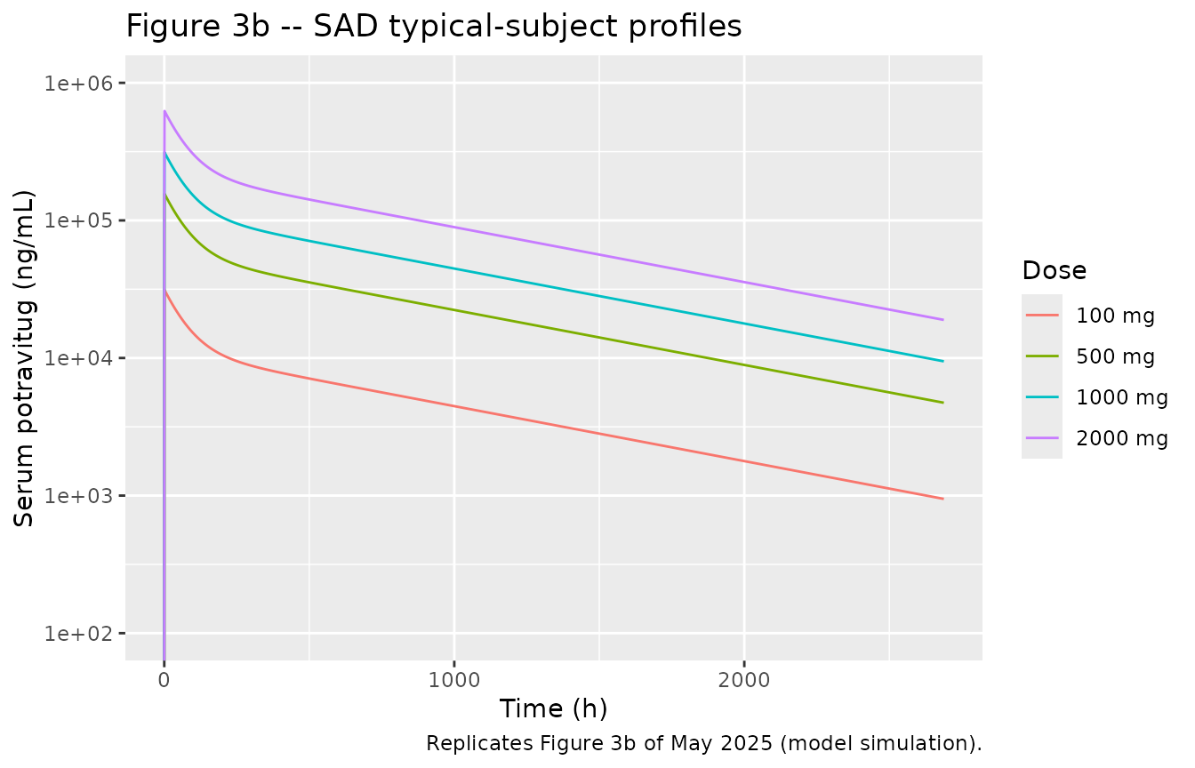
Replicates Figure 3a/b of May 2025: SAD serum potravitug (semi-log).
PKNCA against paper Table 3 (SAD)
NCA uses the protocol sampling times (pre-dose; 1, 2, 6, 12, 24 h; Days 8, 29 and 113), so terminal half-life and AUC extrapolation are estimated from the same points as in the trial.
sad_samples <- c(0, 1, 2, 6, 12, 24, 7 * 24, 28 * 24, 112 * 24)
sad_nca_conc <- sad |>
  dplyr::filter(!is.na(Cc), time %in% sad_samples) |>
  dplyr::select(id, time, Cc, treatment)
stopifnot(nrow(sad_nca_conc) == length(sad_samples) * length(sad_doses))
sad_nca_dose <- sad_ev |>
  dplyr::filter(evid != 0) |>
  dplyr::mutate(treatment = factor(paste(dose, "mg"), levels = paste(sad_doses, "mg"))) |>
  dplyr::select(id, time, amt, dur, treatment)

sad_conc_obj <- PKNCA::PKNCAconc(sad_nca_conc, Cc ~ time | treatment + id)
sad_dose_obj <- PKNCA::PKNCAdose(sad_nca_dose, amt ~ time | treatment + id, duration = "dur", route = "intravascular")
sad_intervals <- data.frame(
  start = 0, end = Inf,
  cmax = TRUE, aucinf.obs = TRUE, half.life = TRUE, cl.obs = TRUE
)
sad_nca <- PKNCA::pk.nca(PKNCA::PKNCAdata(sad_conc_obj, sad_dose_obj, intervals = sad_intervals))

# Paper Table 3, geometric means, converted to ug/mL, h*ug/mL and L/h.
sad_published <- tibble::tribble(
  ~treatment, ~cmax, ~aucinf.obs, ~half.life, ~cl.obs,
  "100 mg", 34.8, 12600, 721.88, 0.007920,
  "500 mg", 170, 78500, 733.22, 0.006369,
  "1000 mg", 341, 132000, 641.42, 0.00756,
  "2000 mg", 631, 261000, 617.79, 0.007667
)
sad_cmp <- nlmixr2lib::ncaComparisonTable(
  simulated = sad_nca,
  reference = sad_published,
  by = "treatment",
  units = c(cmax = "ug/mL", aucinf.obs = "h*ug/mL", half.life = "h", cl.obs = "L/h"),
  tolerance_pct = 20
)
knitr::kable(sad_cmp, caption = "SAD: simulated typical subject vs. paper Table 3 geometric means. * differs by >20%.")| NCA parameter | treatment | Reference | Simulated | % diff |
|---|---|---|---|---|
| Cmax (ug/mL) | 100 mg | 34.8 | 31.2 | -10.3% |
| Cmax (ug/mL) | 500 mg | 170 | 156 | -8.2% |
| Cmax (ug/mL) | 1000 mg | 341 | 312 | -8.5% |
| Cmax (ug/mL) | 2000 mg | 631 | 624 | -1.1% |
| AUC0-∞ (obs) (h*ug/mL) | 100 mg | 12600 | 14000 | +10.9% |
| AUC0-∞ (obs) (h*ug/mL) | 500 mg | 78500 | 69900 | -11.0% |
| AUC0-∞ (obs) (h*ug/mL) | 1000 mg | 132000 | 140000 | +5.9% |
| AUC0-∞ (obs) (h*ug/mL) | 2000 mg | 261000 | 280000 | +7.1% |
| t½ (h) | 100 mg | 722 | 714 | -1.1% |
| t½ (h) | 500 mg | 733 | 714 | -2.6% |
| t½ (h) | 1000 mg | 641 | 714 | +11.3% |
| t½ (h) | 2000 mg | 618 | 714 | +15.6% |
| CL/F (L/h) | 100 mg | 0.00792 | 0.00716 | -9.7% |
| CL/F (L/h) | 500 mg | 0.00637 | 0.00716 | +12.3% |
| CL/F (L/h) | 1000 mg | 0.00756 | 0.00716 | -5.4% |
| CL/F (L/h) | 2000 mg | 0.00767 | 0.00716 | -6.7% |
sad_sim_wide <- as.data.frame(sad_nca) |>
  dplyr::filter(PPTESTCD %in% c("cmax", "aucinf.obs")) |>
  dplyr::select(treatment, PPTESTCD, PPORRES) |>
  tidyr::pivot_wider(names_from = PPTESTCD, values_from = PPORRES) |>
  dplyr::mutate(treatment = as.character(treatment)) |>
  dplyr::inner_join(sad_published, by = "treatment", suffix = c("_sim", "_pub"))
stopifnot(
  nrow(sad_sim_wide) == 4,
  # Calibration data: the typical-subject curve should land within 20% of
  # every cohort's geometric-mean Cmax and AUCinf (n = 3 per cohort).
  all(abs(sad_sim_wide$cmax_sim / sad_sim_wide$cmax_pub - 1) < 0.20),
  all(abs(sad_sim_wide$aucinf.obs_sim / sad_sim_wide$aucinf.obs_pub - 1) < 0.20)
)
Simulated Cmax is 1-10% below the cohort means, AUCinf is within 6-11%, and the terminal half-life (714 h from the Day 29-113 samples) is within 16%; the model’s dose-normalised exposure is constant (linear PK at these doses, since VP1 is femtomolar to picomolar), whereas the observed 500 mg cohort had a somewhat higher dose-normalised AUC than the others.
Unit of Tdist
Table S1 prints Tdist Potravitug = 52.4 without a unit.
Reading it in hours reproduces both the published Cmax and AUC. In
minutes, distribution would be complete within the infusion: Cmax falls
about 28% below the published value and the 24 h concentration (about 11
ug/mL) is far below the roughly 25-30 ug/mL plotted for the first day in
Figure 3b, which shows a distribution phase lasting days. In days, the
AUC doubles. Hours is therefore the only consistent interpretation; it
is also the unit the Applied BioMath platform uses for
Tdist, as in the Marcantonio_2022_*
models.
tdist_sens <- lapply(c(hours = 52.4, minutes = 52.4 / 60, days = 52.4 * 24), function(td) {
  s <- as.data.frame(rxode2::rxSolve(ui, make_sad(100, 1L), params = c(ltdist_ab = log(td))))
  data.frame(
    cmax_ug_ml = max(s$Cc),
    c24h_ug_ml = s$Cc[s$time == 24],
    auc0_2688_h_ug_ml = sum(diff(s$time) * (head(s$Cc, -1) + tail(s$Cc, -1)) / 2)
  )
})
tdist_tab <- dplyr::bind_rows(tdist_sens, .id = "Tdist unit")
knitr::kable(tdist_tab, digits = 1, caption = "100 mg SAD under each candidate Tdist unit. Paper Table 3: Cmax 34.8 ug/mL, AUClast 11700 h.ug/mL.")| Tdist unit | cmax_ug_ml | c24h_ug_ml | auc0_2688_h_ug_ml |
|---|---|---|---|
| hours | 31.2 | 25.4 | 12576.7 |
| minutes | 25.1 | 11.0 | 11178.3 |
| days | 31.3 | 30.4 | 24580.9 |
stopifnot(
  # Hours: Cmax and AUC both within 20% of Table 3.
  abs(tdist_tab$cmax_ug_ml[1] / 34.8 - 1) < 0.20,
  abs(tdist_tab$auc0_2688_h_ug_ml[1] / 11700 - 1) < 0.20,
  # Minutes: Cmax misses by more than 20%; days: AUC misses by more than 50%.
  abs(tdist_tab$cmax_ug_ml[2] / 34.8 - 1) > 0.20,
  abs(tdist_tab$auc0_2688_h_ug_ml[3] / 11700 - 1) > 0.5
)
Multiple ascending dose and dose selection
mad_doses <- c(500, 1000, 2000)
mad_grid <- sort(unique(c(
  seq(0, 52 * 168, by = 6),
  as.vector(outer(c(0, 1, 2, 6, 12, 24), 672 * (0:3), "+"))
)))
make_mad <- function(dose, id) {
  rxode2::et(amt = dose, dur = 1, cmt = "central", ii = 672, addl = 3) |>
    rxode2::et(mad_grid, cmt = "central") |>
    as.data.frame() |>
    dplyr::mutate(id = id, dose = dose)
}
mad_ev <- dplyr::bind_rows(lapply(seq_along(mad_doses), function(i) make_mad(mad_doses[i], i)))
mad <- as.data.frame(rxode2::rxSolve(ui, mad_ev, keep = "dose")) |>
  dplyr::mutate(
    treatment = factor(paste(dose, "mg"), levels = paste(mad_doses, "mg")),
    week = time / 168
  )
mad |>
  dplyr::select(week, treatment, Cc, Ckidney) |>
  tidyr::pivot_longer(c(Cc, Ckidney), names_to = "site", values_to = "conc") |>
  dplyr::mutate(site = dplyr::recode(site, Cc = "(a) Central (blood)", Ckidney = "(b) Kidney interstitial space")) |>
  ggplot(aes(week, conc * 1000, colour = treatment)) +
  geom_line() +
  geom_hline(yintercept = 0.16, linetype = "dotted") +
  facet_wrap(~site) +
  scale_y_log10(limits = c(1e-2, 1e6)) +
  labs(
    x = "Time (weeks)", y = "Potravitug (ng/mL)", colour = "Dose",
    caption = "Dotted line: 0.16 ng/mL = 10 x in vitro IC50. Replicates Figure 4a/b of May 2025."
  )
#> Warning in scale_y_log10(limits = c(0.01, 1e+06)): log-10 transformation
#> introduced infinite values.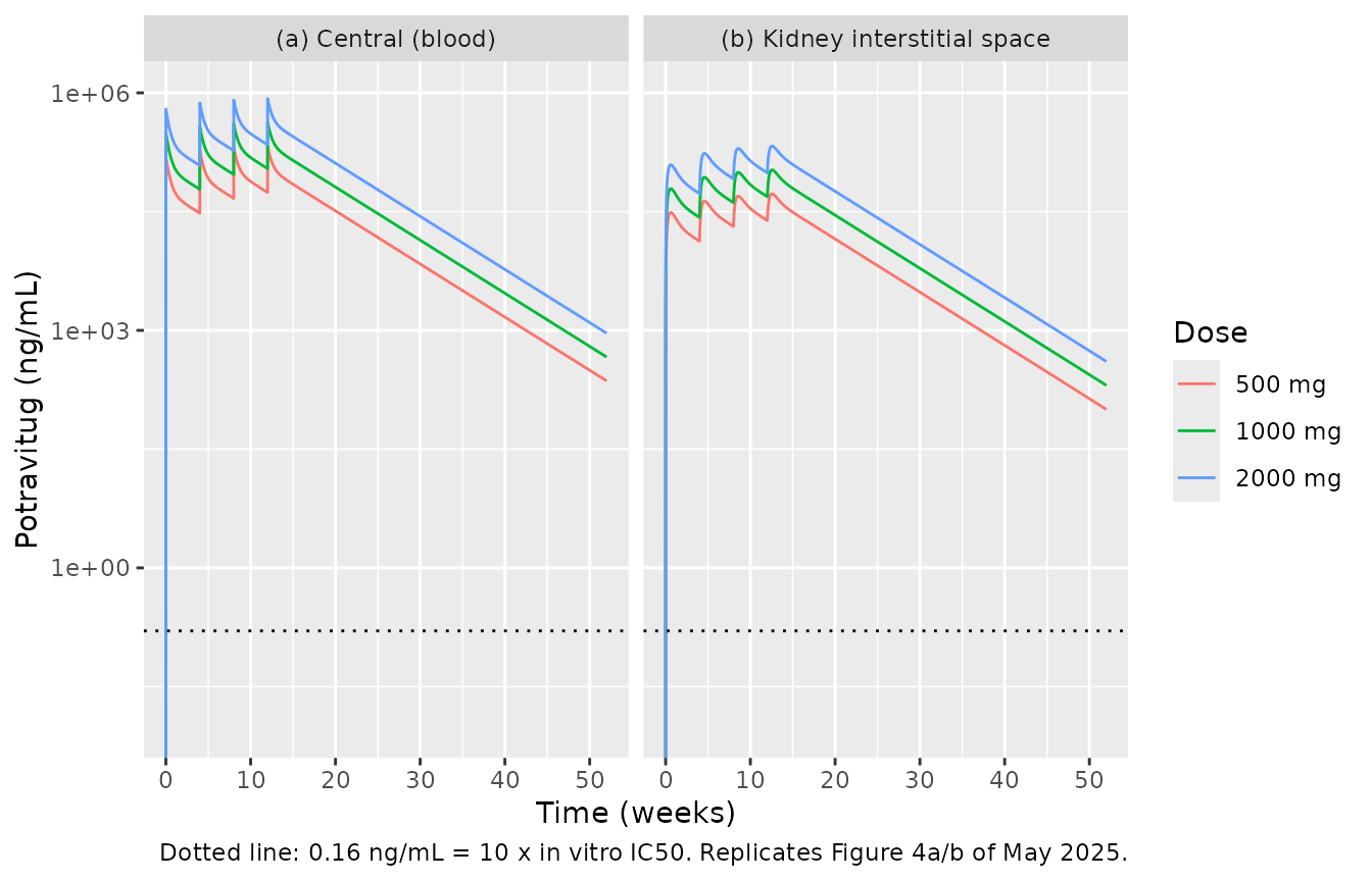
Replicates Figure 4a/b of May 2025: potravitug in blood and in the kidney interstitial space, 4 doses every 4 weeks.
ggplot(mad, aes(week, ro_kidney, colour = treatment)) +
  geom_line() +
  coord_cartesian(ylim = c(95, 100)) +
  labs(
    x = "Time (weeks)", y = "KIS VP1 RO (%)", colour = "Dose",
    caption = "Replicates Figure 4c of May 2025."
  )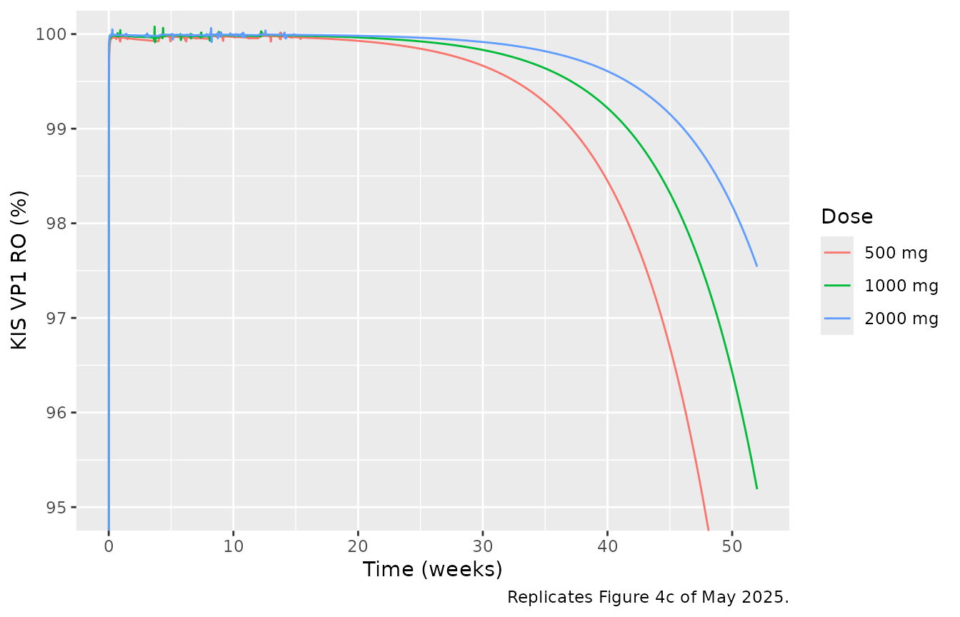
Replicates Figure 4c of May 2025: VP1 receptor occupancy in the kidney interstitial space.
The paper’s dose-selection claim is that 1000 mg every 4 weeks x 4 keeps the KIS potravitug concentration above 0.16 ng/mL and KIS VP1 occupancy above 95% for 52 weeks; Figure 4c shows the 500 mg curve reaching 95% at about week 48 and the 2000 mg curve ending near 97.5%. The simulation reproduces all three (table and week below).
ro_52 <- mad |>
  dplyr::filter(time == 52 * 168) |>
  dplyr::select(treatment, Cc, Ckidney, ro_blood, ro_kidney)
knitr::kable(ro_52, digits = 3, caption = "Week 52 after the first of four doses.")| treatment | Cc | Ckidney | ro_blood | ro_kidney |
|---|---|---|---|---|
| 500 mg | 0.230 | 0.100 | 95.757 | 90.775 |
| 1000 mg | 0.460 | 0.202 | 97.832 | 95.189 |
| 2000 mg | 0.921 | 0.405 | 98.904 | 97.542 |
week_ro95_500 <- mad |>
  dplyr::filter(dose == 500, week > 1, ro_kidney < 95) |>
  dplyr::summarise(week = min(week)) |>
  dplyr::pull(week)
week_ro95_500
#> [1] 47.78571
stopifnot(
  # Deterministic typical-subject solve: these are fixed numbers, not draws.
  ro_52$ro_kidney[ro_52$treatment == "1000 mg"] > 95,
  ro_52$ro_kidney[ro_52$treatment == "2000 mg"] > 97 && ro_52$ro_kidney[ro_52$treatment == "2000 mg"] < 98.5,
  week_ro95_500 > 44 && week_ro95_500 < 52,
  all(ro_52$Ckidney * 1000 > 0.16)
)
Potravitug binds VP1 far faster (kon x free antibody, several per
hour even at week 52) than free antibody changes, so the complex sits at
its binding quasi-steady state. Setting d/dt(complex) = 0
gives RO = Ab / (Ab + Kss) with
Kss = Kd + kdeg_VP1 / kon (60 pM + 8 pM, the second term
because bound potravitug is cleared with VP1). This relation does not
involve the VP1 synthesis rate, so it also shows that how VP1 is
supplied (see Assumptions) does not move the occupancy prediction. The
check below confirms it in the KIS after the first week.
mw <- ini_vals[["mw"]]
kon_nm_h <- ini_vals[["kon"]] * 3600
kdeg_vp1 <- log(2) / (exp(ini_vals[["lthalf_vp1"]]) / 60)
kss_nm <- ini_vals[["kd"]] / 1000 + kdeg_vp1 / kon_nm_h
ro_eq <- mad |>
  dplyr::filter(time >= 168) |>
  dplyr::mutate(
    ab_kidney_nm = Ckidney * 1e6 / mw,
    ro_qss = 100 * ab_kidney_nm / (ab_kidney_nm + kss_nm)
  )
max_dev <- max(abs(ro_eq$ro_kidney - ro_eq$ro_qss))
max_dev
#> [1] 0.116084
# Same solve on both sides; the residual is the short lag while free drug
# rises during each infusion.
stopifnot(max_dev < 0.15)
PKNCA against paper Table 3 (MAD, Day 85)
The MAD cohorts were the model’s external validation set. Day 85 (fourth dose, t = 2016 h) Cmax and AUC over the 672 h dosing interval are compared with the published geometric means; the trough is the pre-dose concentration on Day 85, compared with the published median.
mad_nca_conc <- mad |>
  dplyr::filter(!is.na(Cc), time >= 2016, time <= 2688) |>
  dplyr::select(id, time, Cc, treatment)
mad_nca_dose <- mad_ev |>
  dplyr::filter(evid != 0) |>
  dplyr::mutate(treatment = factor(paste(dose, "mg"), levels = paste(mad_doses, "mg"))) |>
  dplyr::select(id, time, amt, dur, treatment)
mad_conc_obj <- PKNCA::PKNCAconc(mad_nca_conc, Cc ~ time | treatment + id)
mad_dose_obj <- PKNCA::PKNCAdose(mad_nca_dose, amt ~ time | treatment + id, duration = "dur", route = "intravascular")
mad_intervals <- data.frame(start = 2016, end = 2688, cmax = TRUE, auclast = TRUE)
mad_nca <- PKNCA::pk.nca(PKNCA::PKNCAdata(mad_conc_obj, mad_dose_obj, intervals = mad_intervals))

mad_trough <- mad |>
  dplyr::filter(time == 2016) |>
  dplyr::select(treatment, PPORRES = Cc) |>
  dplyr::mutate(PPTESTCD = "ctrough")
mad_sim <- dplyr::bind_rows(
  as.data.frame(mad_nca) |> dplyr::select(treatment, PPTESTCD, PPORRES),
  mad_trough
)
mad_published <- tibble::tribble(
  ~treatment, ~cmax, ~auclast, ~ctrough,
  "500 mg", 253, 57200, 50.3,
  "1000 mg", 487, 126000, 84.5,
  "2000 mg", 868, 230000, 198
)
mad_cmp <- nlmixr2lib::ncaComparisonTable(
  simulated = mad_sim,
  reference = mad_published,
  by = "treatment",
  units = c(cmax = "ug/mL", auclast = "h*ug/mL", ctrough = "ug/mL"),
  tolerance_pct = 20
)
knitr::kable(mad_cmp, caption = "MAD Day 85: simulated typical subject vs. paper Table 3. AUC is AUCtau (672 h). * differs by >20%.")| NCA parameter | treatment | Reference | Simulated | % diff |
|---|---|---|---|---|
| Cmax (ug/mL) | 500 mg | 253 | 211 | -16.5% |
| Cmax (ug/mL) | 1000 mg | 487 | 422 | -13.3% |
| Cmax (ug/mL) | 2000 mg | 868 | 845 | -2.7% |
| AUClast (h*ug/mL) | 500 mg | 57200 | 62900 | +9.9% |
| AUClast (h*ug/mL) | 1000 mg | 126000 | 126000 | -0.2% |
| AUClast (h*ug/mL) | 2000 mg | 230000 | 252000 | +9.4% |
| Ctrough (ug/mL) | 500 mg | 50.3 | 55.3 | +9.9% |
| Ctrough (ug/mL) | 1000 mg | 84.5 | 111 | +30.8%* |
| Ctrough (ug/mL) | 2000 mg | 198 | 221 | +11.7% |
Day 85 Cmax is within 17% and AUCtau within 10% at every dose. The trough is within 12% at 500 and 2000 mg and 31% above the published median at 1000 mg (a median of 5 participants, whose own range, 77.8-119 ug/mL, contains the simulated 111 ug/mL).
Assumptions and deviations
-
Unit of
Tdist. Table S1 givesTdist Potravitug = 52.4with no unit. Hours is used: it is the only reading that reproduces the published SAD Cmax and AUC (see “Unit ofTdist” above) and is the unit used by the same modelling platform forTdistelsewhere in this library. - Potravitug molar mass. The paper does not state it. A typical IgG1 value of 150 kDa is used to convert mass concentrations to nM for binding. It affects only the occupancy outputs, and with it the model reproduces the week-52 occupancies read from Figure 4c (about 95% at 1000 mg and 97.5% at 2000 mg).
- VP1 supply between kidney and blood. Table S1 says VP1 synthesis and kidney-to-blood distribution “is described using an analytical solution that results in a VP1 concentration in the kidney that is 1000-fold higher than blood”, without giving a transport rate. The maintainers implement that analytical solution as a constant (zero-order) VP1 input into each compartment equal to its baseline degradation, which uses only tabulated values and holds the 1000-fold ratio exactly. Free and bound VP1 are not exchanged between compartments in this implementation. Because potravitug binding is far faster than VP1 turnover, occupancy equals its binding equilibrium regardless of how VP1 is supplied (checked above), and VP1 is too dilute (fM-pM) to affect potravitug PK.
-
Shared distribution parameters. Table S1 lists a
single
PdistandTdistfor potravitug, and its Model Assumptions apply them to “the peripheral tissues (including kidney)”; both tissue exchanges use them. -
konunits. The Model Assumptions text writeskon = 0.001 sec-1; the Table S1 row gives the dimensionally correct1/nM/s, which is used. - Infusion duration. Not stated; 1 h is used (Tmax at the 1 h sample).
- No IIV or residual error. The model was fitted to cohort means for a typical 70 kg subject, so none is reported or encoded.
- Table 1 race row. The SAD-placebo Asian entry is split across two rows in the published table (“2” and “(50.0%)”); it is read as 2 Asian participants, which makes the race counts sum to 40.
- No erratum or correction notice for this article was found (checked 2026-11-05).