Gamma-hydroxybutyric acid, rat (Felmlee 2010)
Source:vignettes/articles/Felmlee_2010_ghb_rat.Rmd
Felmlee_2010_ghb_rat.RmdModel and source
- Citation: Felmlee MA, Wang Q, Cui D, Roiko SA, Morris ME. Mechanistic toxicokinetic model for gamma-hydroxybutyric acid: inhibition of active renal reabsorption as a potential therapeutic strategy. The AAPS Journal. 2010;12(3):407-416. doi:10.1208/s12248-010-9197-x.
- Description: Preclinical (rat). Mechanistic hybrid-physiological toxicokinetic model for gamma-hydroxybutyric acid (GHB) in male Sprague-Dawley rats after intravenous bolus doses of 200 to 1,000 mg/kg, fitting plasma concentrations and cumulative urinary excretion simultaneously. Disposition is a plasma compartment exchanging with two tissue compartments (fast and slow) by distributional clearances, plus a kidney compartment perfused at renal blood flow. Capacity-limited metabolic elimination (Michaelis-Menten) acts on the first tissue compartment. Drug is filtered from the kidney compartment at the glomerular filtration rate into a proximal-tubule ultrafiltrate compartment, from which it is actively reabsorbed back into the kidney by a saturable (Michaelis-Menten) monocarboxylate-transporter process; the surviving filtrate flows at the urine flow rate through a distal-tubule ultrafiltrate compartment into the cumulative urine compartment. Plasma volume, kidney volume, both ultrafiltrate volumes, renal blood flow and urine flow were fixed to rat physiological values. The saturable reabsorption term carries an optional monocarboxylate-transporter inhibition extension (source paper Eqs. 11-13) that reproduces the paper’s competitive, noncompetitive and uncompetitive inhibition simulations; with the two inhibition covariates at their default of zero the term reduces exactly to the fitted model (source paper Eq. 4). Fit by NONMEM VI ADVAN9 with FOCE.
- Article: https://doi.org/10.1208/s12248-010-9197-x
Felmlee and colleagues built the first mechanistic toxicokinetic (TK) model for gamma-hydroxybutyric acid (GHB) that carries both of the drug’s nonlinearities at once: capacity-limited metabolism and saturable active renal reabsorption. The motivating question is therapeutic. GHB overdose has no antidote; because reabsorption from the proximal tubule is monocarboxylate-transporter (MCT) mediated and saturable, inhibiting it should increase renal clearance and lower plasma exposure. The paper uses the fitted model to simulate that intervention and then corroborates the prediction experimentally with L-lactate, a known MCT inhibitor.
mod <- rxode2::rxode(readModelDb("Felmlee_2010_ghb_rat"))
#> ℹ parameter labels from comments will be replaced by 'label()'
Population
| Field | Value |
|---|---|
| Species | rat (male Sprague-Dawley) |
| N | 34 (7-10 per dose group) |
| Weight | 280-320 g |
| Doses | 200, 400, 600 or 1,000 mg/kg, single IV bolus (jugular vein) |
| Sampling | Plasma 0-360 min (12 points); urine 0-60, 60-120, 120-240, 240-360 min |
| Region | USA (University at Buffalo) |
Male Sprague-Dawley rats (Harlan), 280-320 g, cannulated in the right jugular vein and housed in metabolic cages. GHB in plasma and urine was measured by LC/MS/MS. Plasma concentration and cumulative urinary excretion from all four doses were fitted simultaneously in NONMEM VI (level 1.1) using FOCE and the ADVAN9 differential-equation solver (source paper Methods, “Population TK Modeling”).
A separate interaction study (GHB 600 mg/kg alone, N = 3, versus GHB 600 mg/kg plus L-lactate 330 mg/kg IV bolus with a 121 mg/kg/h IV infusion, N = 5) was run to confirm the inhibition simulations; it did not contribute to the model fit.
Structural model
The model is hybrid physiological (semi-PBPK): several volumes and flows are fixed to rat physiological values and the remaining nonlinear parameters are estimated.
-
central(plasma) exchanges withperipheral1(fast tissue) andperipheral2(slow tissue) at distributional clearances CLD and CLD2. - Capacity-limited metabolic elimination
(Michaelis-Menten) acts on
peripheral1, not on plasma. -
centralexchanges withkidneyat renal blood flow QR, and drug is filtered out ofkidneyat GFR intoulf1, the proximal-tubule ultrafiltrate. - Saturable active reabsorption (MCT-mediated,
Michaelis-Menten) returns drug from
ulf1tokidney. Reabsorption occurs from the proximal tubule only. - Urine flow UF carries the surviving filtrate
ulf1->ulf2(distal tubule) ->urine. The distal compartment exists to reproduce the delay between filtration at the glomerulus and the appearance of drug in voided urine.
The two ultrafiltrate states are declared through the documented
paper_specific_compartments escape hatch, because
ulf1 / ulf2 are specific to renal-tubule
models rather than library-wide canonical compartments.
Transport-inhibition extension
Source paper Eqs. 11-13 modify the reabsorption rate law for a
steady-state inhibitor at ratio R = [I] / Ki. The packaged
model encodes all three mechanisms in one branch-free expression using
two multiplier covariates:
reabsorption <- vmax_reab /
(km_reab * (1 + INH_MCT_KM_RATIO) + Culf1 * (1 + INH_MCT_CONC_RATIO))| Mechanism | INH_MCT_KM_RATIO | INH_MCT_CONC_RATIO |
|---|---|---|
| None (fitted model, Eq. 4) | 0 | 0 |
| Competitive (Eq. 11) | R | 0 |
| Noncompetitive (Eq. 12) | R | R |
| Uncompetitive (Eq. 13) | 0 | R |
Both covariates default to 0, so a user who never sets them recovers the fitted model exactly. Only the competitive case is tabulated by the paper (Table II and Fig. 3); the noncompetitive and uncompetitive results are reported as “data not shown”.
Source trace
Every equation and every ini() value, with its location
in the source paper.
| Item | Source | Value |
|---|---|---|
| d/dt(central) | Eq. 1 | -(QR + CLD + CLD2)Cc + QRCk + CLDCp1 + CLD2Cp2 |
| d/dt(peripheral1) | Eq. 2 | CLDCc - (CLD + Vmax,m/(Km,m + Cp1))Cp1 |
| d/dt(peripheral2) | Eq. 3 | CLD2Cc - CLD2Cp2 |
| Reabsorption | Eq. 4 | Vmax,R / (Km,R + Culf1) [a clearance] |
| d/dt(kidney) | Eq. 5 | QRCc - (QR + GFR)Ck + Reabsorption*Culf1 |
| d/dt(ulf1) | Eq. 6 | GFRCk - UFCulf1 - Reabsorption*Culf1 |
| d/dt(ulf2) | Eq. 7 | UFCulf1 - UFCulf2 |
| d/dt(urine) | Eq. 8 | UF*Culf2 |
| Plasma residual error | Eq. 9 | Y = Log(Aplasma/Vplasma) + eps_plasma |
| Urine residual error | Eq. 10 | Y = Log(Aurine) + eps_urine |
| Competitive inhibition | Eq. 11 | Km,R * (1 + R) |
| Noncompetitive inhibition | Eq. 12 | Km,R * (1 + R), Culf1 * (1 + R) |
| Uncompetitive inhibition | Eq. 13 | Culf1 * (1 + R) |
| Time-averaged renal clearance | Eq. 14 | CLR = Ae,inf / AUC_plasma |
| lvc (Vplasma) | Table I | 10.5 mL, FIXED (footnote a) |
| lvp (Vtissue1) | Table I | 75.9 mL (16% CV) |
| lvp2 (Vtissue2) | Table I | 26.8 mL |
| lv_kidney (Vkidney) | Table I | 4.0 mL, FIXED (footnote a) |
| lv_ulf1 (Vulf1) | Table I | 3.0 mL, FIXED (footnote a) |
| lv_ulf2 (Vulf2) | Table I | 1.0 mL, FIXED (footnote a) |
| lq (CLD) | Table I | 26.9 mL/min |
| lq2 (CLD2) | Table I | 3.07 mL/min |
| lq_kidney (QR) | Table I | 12.5 mL/min, FIXED (footnote a) |
| lvmax (Vmax,m) | Table I | 0.581 mg/min |
| lkm (Km,m) | Table I | 0.054 mg/mL |
| lgfr (GFR) | Table I | 10 mL/min/kg (see Errata) |
| lvmax_reab (Vmax,R) | Table I | 2.34 mg/min |
| lkm_reab (Km,R) | Table I | 0.46 mg/mL |
| luf (UF) | Table I | 0.1 mL/min, FIXED (footnote a) (114% CV) |
| expSd (eps_plasma) | Table I | 2.5% |
| expSd_urine (eps_urine) | Table I | 46% |
Between-subject variability is exponential
(P_i = theta * exp(eta_i), source paper “Structural,
Parameter Variability, and Observational Models”), reported in Table I
as CV% on exactly two parameters. The packaged model uses
omega^2 = log(1 + CV^2), the same convention as the
companion rat GHB model already in the library,
Fung_2008_butanediol_rat.R, whose variability reporting
this paper explicitly says it followed (source paper reference 26).
Simulation setup
WT_KG   <- 0.3                       # 280-320 g study rats; see Errata
DOSES   <- c(200, 400, 600, 1000)    # mg/kg
R_LEVEL <- c(0, 1, 10, 100)          # [I]/Ki for competitive inhibition
NSUB    <- 200                       # per arm; the paper simulated 1,000

# Route A event table (ODE-state cmt + explicit dvid). This model declares two
# endpoints (Cc and urine), so every observation row must say which endpoint it
# belongs to: dvid 1 = plasma concentration, dvid 2 = cumulative urine amount.
build_events <- function(dose_mgkg, r_km = 0, r_conc = 0,
                         tgrid = seq(0, 360, by = 1), both_endpoints = FALSE) {
  obs <- data.frame(
    time = tgrid, amt = NA_real_, evid = 0L, cmt = "central", dvid = 1L
  )
  if (both_endpoints) {
    obs <- rbind(obs, transform(obs, dvid = 2L))
  }
  ev <- rbind(
    data.frame(
      time = 0, amt = dose_mgkg * WT_KG, evid = 1L,
      cmt = "central", dvid = NA_integer_
    ),
    obs
  )
  ev <- ev[order(ev$time, -ev$evid), ]
  ev$WT <- WT_KG
  ev$INH_MCT_KM_RATIO <- r_km
  ev$INH_MCT_CONC_RATIO <- r_conc
  ev
}

# Trapezoidal AUC, matching the paper's WinNonLin linear-trapezoidal AUC.
trap_auc <- function(time, conc) {
  sum(diff(time) * (utils::head(conc, -1) + utils::tail(conc, -1)) / 2)
}
Reproducing Table II: plasma AUC under competitive inhibition
Table II is the paper’s central quantitative result: plasma AUC and
time-averaged renal clearance for each of the four doses, with no
inhibitor and at R = 1, 10 and 100. The AUC column is the
load-bearing check on the transcription, because it depends on every
ODE, every Table I parameter, the dose/body-weight bridge and the
competitive-inhibition rate law at once.
Sixteen typical-value (no random effects) solves, one per dose x
R cell:
scen <- tidyr::expand_grid(dose = DOSES, R = R_LEVEL) |>
  dplyr::mutate(id = dplyr::row_number())

ev_all <- do.call(rbind, lapply(seq_len(nrow(scen)), function(i) {
  e <- build_events(scen$dose[i], r_km = scen$R[i], tgrid = seq(0, 360, by = 0.5))
  e$id <- scen$id[i]
  e
}))

sim_tv <- rxode2::rxSolve(
  mod, ev_all, returnType = "data.frame",
  omega = NA, sigma = NA, addDosing = FALSE
)

auc_tv <- sim_tv |>
  dplyr::filter(!is.na(Cc)) |>
  dplyr::group_by(id) |>
  dplyr::summarise(
    auc = trap_auc(time, Cc),
    ae  = max(urine),
    .groups = "drop"
  ) |>
dplyr::left_join(scen, by = "id")| GHB dose (mg/kg) | R = [I]/Ki | Published AUC | Simulated AUC | % diff |
|---|---|---|---|---|
| 200 | 0 | 29.3 | 31.2 | 6.4 |
| 200 | 1 | 27.4 | 29.3 | 7.1 |
| 200 | 10 | 21.0 | 22.6 | 7.7 |
| 200 | 100 | 14.4 | 15.7 | 9.0 |
| 400 | 0 | 83.0 | 87.5 | 5.5 |
| 400 | 1 | 76.2 | 80.4 | 5.5 |
| 400 | 10 | 56.6 | 58.9 | 4.1 |
| 400 | 100 | 37.5 | 38.9 | 3.8 |
| 600 | 0 | 133.3 | 135.2 | 1.5 |
| 600 | 1 | 124.6 | 126.3 | 1.4 |
| 600 | 10 | 96.1 | 96.4 | 0.3 |
| 600 | 100 | 63.6 | 64.8 | 1.8 |
| 1000 | 0 | 208.2 | 208.9 | 0.3 |
| 1000 | 1 | 198.8 | 200.0 | 0.6 |
| 1000 | 10 | 165.2 | 165.7 | 0.3 |
| 1000 | 100 | 117.1 | 119.0 | 1.7 |
# Deterministic typical-value solves: no random draws on either side, so a
# tight bound is reproducible across rxode2 builds.
stopifnot(
  median(abs(chk_auc$pct_diff)) < 6,
  max(abs(chk_auc$pct_diff)) < 12
)
All sixteen cells agree with the published values, and the agreement
is tightest at the two highest doses, which carry the most informative
data. The AUC falls monotonically with increasing R at
every dose, reproducing the paper’s headline claim that inhibiting
reabsorption lowers GHB exposure.
Reproducing Figure 3: profiles under competitive inhibition
sim_tv |>
  dplyr::filter(!is.na(Cc)) |>
  dplyr::left_join(scen, by = "id") |>
  dplyr::mutate(
    dose_lab = factor(paste0(format(dose, big.mark = ","), " mg/kg"),
                      levels = paste0(format(DOSES, big.mark = ","), " mg/kg")),
    R_lab = factor(R, levels = R_LEVEL,
                   labels = c("no inhibitor", "R = 1", "R = 10", "R = 100"))
  ) |>
  ggplot2::ggplot(ggplot2::aes(time, Cc, colour = R_lab, linetype = R_lab)) +
  ggplot2::geom_line(linewidth = 0.7) +
  ggplot2::facet_wrap(~dose_lab, scales = "free_y") +
  ggplot2::scale_y_log10() +
  ggplot2::labs(
    x = "Time (min)", y = "GHB plasma concentration (mg/mL)",
    colour = NULL, linetype = NULL
  ) +
  ggplot2::theme_bw() +
  ggplot2::theme(legend.position = "top")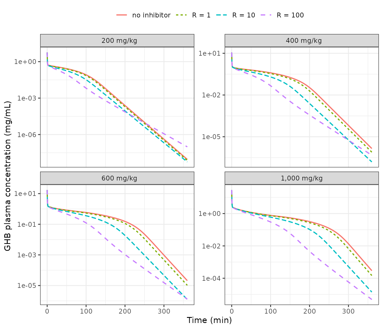
Replicates Figure 3 of Felmlee 2010: simulated plasma GHB concentration-time profiles in the absence and presence of a competitive inhibitor of renal reabsorption.
Reproducing Figure 2: population variability
Figure 2 shows, for each dose, the mean and the 10th and 90th percentiles of 1,000 simulated profiles against the observed data. Two details of that figure govern how it must be reproduced:
- The bands are computed from simulated observations, so they
include the residual error of Eqs. 9-10 (2.5% for plasma, 46% for
urine), not only between-subject variability. In
rxSolve()output the residual-error column issim; theCc/ipredSimcolumns are individual predictions with no residual error. - Urinary excretion carries a 114% CV on urine flow, which makes the distribution of excreted amount strongly right-skewed. The mean line therefore sits well above the median, which is what the published figure shows.
cohort <- do.call(rbind, lapply(DOSES, function(d) {
  ev <- build_events(d, tgrid = seq(0, 360, by = 5), both_endpoints = TRUE)
  rxode2::rxSolve(
    mod, ev, nSub = NSUB, returnType = "data.frame",
    addDosing = FALSE, keep = "dvid"
  ) |>
    dplyr::mutate(dose = d)
}))

bands <- cohort |>
  dplyr::mutate(
    endpoint = ifelse(dvid == 1L, "Plasma (mg/mL)", "Cumulative urine (mg)")
  ) |>
  dplyr::group_by(dose, endpoint, time) |>
  dplyr::summarise(
    mean = mean(sim),
    p10  = quantile(sim, 0.10),
    p90  = quantile(sim, 0.90),
    .groups = "drop"
  )
bands |>
  dplyr::mutate(
    dose_lab = factor(paste0(format(dose, big.mark = ","), " mg/kg"),
                      levels = paste0(format(DOSES, big.mark = ","), " mg/kg"))
  ) |>
  ggplot2::ggplot(ggplot2::aes(time)) +
  ggplot2::geom_ribbon(ggplot2::aes(ymin = p10, ymax = p90), alpha = 0.15) +
  ggplot2::geom_line(ggplot2::aes(y = mean), linewidth = 0.7) +
  ggplot2::geom_line(ggplot2::aes(y = p10), linetype = "dashed", linewidth = 0.3) +
  ggplot2::geom_line(ggplot2::aes(y = p90), linetype = "dashed", linewidth = 0.3) +
  ggplot2::facet_grid(endpoint ~ dose_lab, scales = "free_y") +
  ggplot2::labs(x = "Time (min)", y = NULL) +
  ggplot2::theme_bw()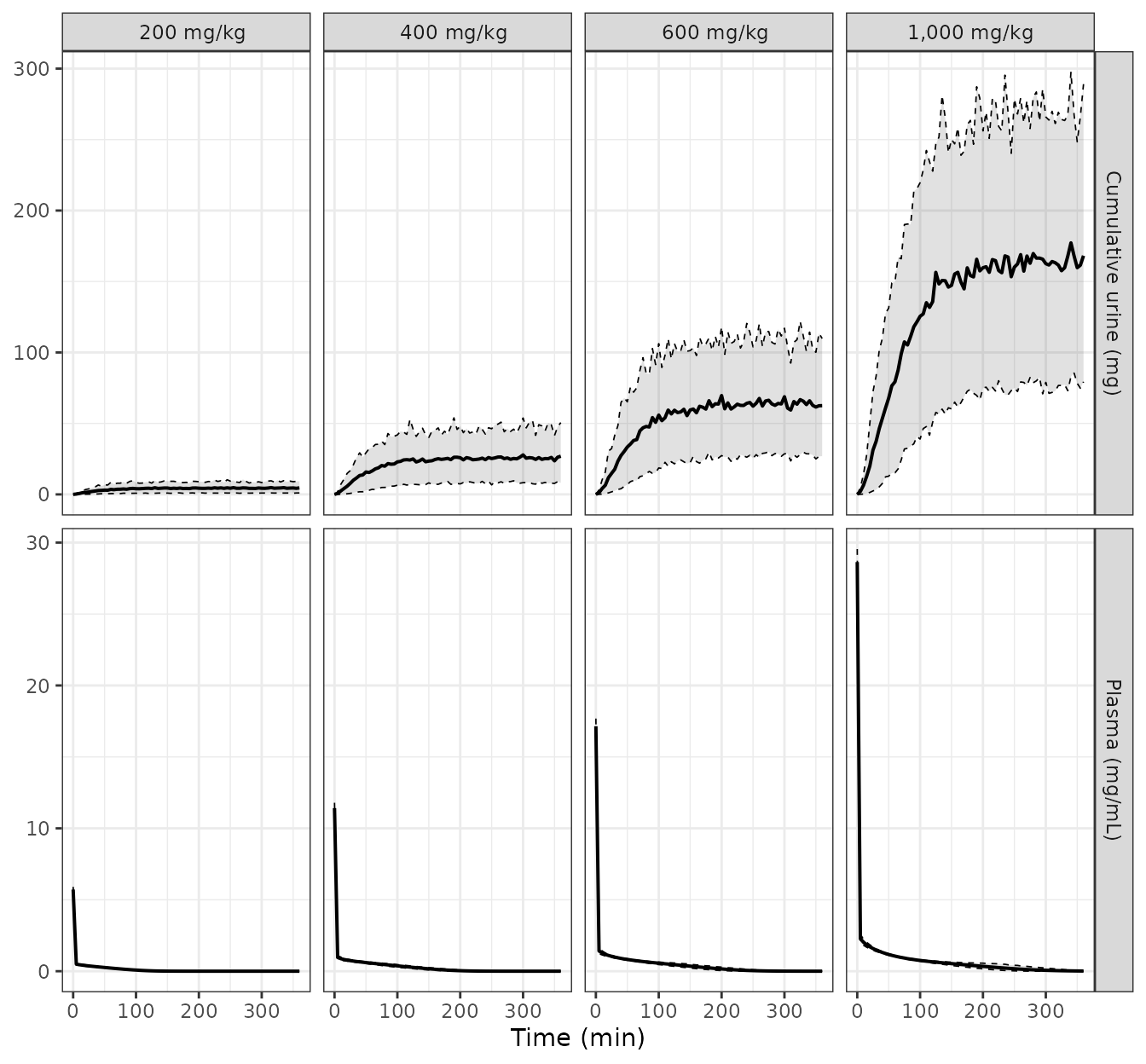
Replicates Figure 2 of Felmlee 2010: mean (solid) with 10th and 90th percentiles (dashed) of simulated plasma concentration and cumulative urinary excretion.
The published Figure 2 mean cumulative urinary excretion at 360 min
reads approximately 5.7, 27.5, 78 and 170 mg at 200, 400, 600 and 1,000
mg/kg. Those values are also recoverable arithmetically from Table II,
since Eq. 14 gives Ae,inf = CLR * AUC: 0.197 x 29.3 = 5.8,
0.331 x 83.0 = 27.5, 0.540 x 133.3 = 72.0 and 0.823 x 208.2 = 171.3 mg.
Three of the four agree closely with the figure; the 600 mg/kg point
differs by about 8% (roughly 78 mg read off the figure against 72.0 mg
from the table), which is within the precision of reading a value off a
log-scaled panel. That correspondence is what identifies both the figure
and the table as reporting population means including residual
error rather than typical values.
ae360 <- cohort |>
  dplyr::filter(dvid == 2L, time == 360) |>
  dplyr::group_by(dose) |>
  dplyr::summarise(mean_ae = mean(sim), .groups = "drop") |>
  dplyr::mutate(
    published_ae = c(29.3, 83.0, 133.3, 208.2) * c(0.197, 0.331, 0.540, 0.823),
    pct_diff = 100 * (mean_ae - published_ae) / published_ae
  )

knitr::kable(
  dplyr::transmute(
    ae360,
    `GHB dose (mg/kg)` = dose,
    `Published Ae,inf (mg)` = round(published_ae, 1),
    `Simulated mean Ae (mg)` = round(mean_ae, 1),
    `% diff` = round(pct_diff, 1)
  ),
  caption = "Cumulative urinary excretion at 360 min, back-calculated from Table II via Eq. 14."
)| GHB dose (mg/kg) | Published Ae,inf (mg) | Simulated mean Ae (mg) | % diff |
|---|---|---|---|
| 200 | 5.8 | 4.4 | -23.7 |
| 400 | 27.5 | 24.1 | -12.1 |
| 600 | 72.0 | 61.2 | -14.9 |
| 1000 | 171.3 | 166.5 | -2.8 |
# A cohort mean over a 114%-CV parameter is a heavy-tailed statistic, so this
# assertion bounds the centre of the comparison rather than any single dose.
stopifnot(median(abs(ae360$pct_diff)) < 40)
The simulated cohort means fall short of the published ones at the lower doses, most at 200 mg/kg, and close the gap as dose rises. This is a reconstruction gap in a derived metric, not a transcription error, and it is discussed under Errata below. Note that the cohort mean of a 114%-CV parameter is a heavy-tailed statistic, so the per-dose percentages move with the random draw; only the centre of the comparison is asserted above.
PKNCA validation
Noncompartmental analysis of the typical-value plasma profiles, on the same 0-360 min window the paper sampled. The NCA is run on the typical-value solve rather than the full-variability cohort: with a 114% CV on urine flow, terminal slopes across a simulated cohort are heterogeneous enough that a pooled half-life is dominated by which subjects happened to draw a slow tubular flow.
# Select the no-inhibitor arms by id up front, so the only row-dropping filter
# in the PKNCA chain below is the mandatory !is.na() one.
tv_ids <- scen$id[scen$R == 0]

nca_conc <- sim_tv[sim_tv$id %in% tv_ids, ] |>
  dplyr::left_join(scen, by = "id") |>
  dplyr::filter(!is.na(Cc)) |>
  dplyr::transmute(
    id = as.integer(id),
    treatment = paste0(format(dose, big.mark = ","), " mg/kg"),
    time, Cc
  )

# PKNCA warns "AUC range starting (0) before the first measurement" once per
# subject if any profile lacks a time-zero record, so assert it rather than
# discovering it in the render log.
stopifnot(all(table(nca_conc$treatment[nca_conc$time == 0]) == 1))

nca_dose <- nca_conc |>
  dplyr::distinct(id, treatment) |>
  dplyr::mutate(time = 0, amt = DOSES * WT_KG)

# Additive grouping (| treatment + id) on BOTH objects: PKNCAdose rejects a
# nested slash formula. `dose` and `route` are reserved PKNCA column names, so
# the grouping column is `treatment`.
o_conc <- PKNCA::PKNCAconc(nca_conc, Cc ~ time | treatment + id,
                           concu = "mg/mL", timeu = "min")
o_dose <- PKNCA::PKNCAdose(nca_dose, amt ~ time | treatment + id, doseu = "mg")

intervals <- data.frame(
  start = 0, end = 360,
  cmax = TRUE, tmax = TRUE, auclast = TRUE, clast.obs = TRUE
)

nca_res <- PKNCA::pk.nca(PKNCA::PKNCAdata(o_conc, o_dose, intervals = intervals))
nca_sum <- as.data.frame(nca_res)| Treatment | AUClast (min*mg/mL) | Cmax (mg/mL) | Tmax (min) | Clast (mg/mL) |
|---|---|---|---|---|
| 200 mg/kg | 30.9 | 5.71 | 0 | 0.00e+00 |
| 400 mg/kg | 87.0 | 11.40 | 0 | 1.40e-06 |
| 600 mg/kg | 134.0 | 17.10 | 0 | 2.08e-05 |
| 1,000 mg/kg | 208.0 | 28.60 | 0 | 2.93e-04 |
Comparison against the published AUC
The paper reports no Cmax / Tmax / half-life table, so the AUC column
of Table II is the only published NCA quantity available for a
side-by-side comparison. It was itself computed by NCA in WinNonLin 5.2
(source paper Methods, “Statistical and Non-Compartmental Analyses”; the
paper does not state which trapezoidal rule was used), so
auclast over 0-360 min is the matching parameter.
ref_nca <- data.frame(
  treatment = paste0(format(DOSES, big.mark = ","), " mg/kg"),
  auclast = c(29.3, 83.0, 133.3, 208.2)
)

cmp <- nlmixr2lib::ncaComparisonTable(
  simulated = nca_sum,
  reference = ref_nca,
  by = "treatment",
  params = "auclast",
  units = c(auclast = "min*mg/mL")
)
knitr::kable(cmp, caption = "Simulated versus published plasma AUC (Felmlee 2010 Table II, GHB alone).")| NCA parameter | treatment | Reference | Simulated | % diff |
|---|---|---|---|---|
| AUClast (min*mg/mL) | 200 mg/kg | 29.3 | 30.9 | +5.4% |
| AUClast (min*mg/mL) | 400 mg/kg | 83 | 87 | +4.8% |
| AUClast (min*mg/mL) | 600 mg/kg | 133 | 134 | +0.8% |
| AUClast (min*mg/mL) | 1,000 mg/kg | 208 | 208 | -0.3% |
attr(cmp, "footnote")
#> NULL
No row exceeds the 20% flagging tolerance.
The L-lactate interaction study (Table III)
Table III reports the experimental confirmation: GHB 600 mg/kg alone
versus the same dose co-administered with L-lactate. The paper notes
that the observed changes resemble the simulated R = 10
case.
| Arm | AUC (min*mg/mL) | CLR (mL/min) | Sleep time (min) |
|---|---|---|---|
| GHB alone (N = 3), observed | 131 +/- 18.8 | 0.415 +/- 0.06 | 126 +/- 15.1 |
| GHB + L-lactate (N = 5), observed | 74.8 +/- 9.4 | 0.910 +/- 0.10 | 87.0 +/- 11.1 |
| GHB alone, simulated | 135.2 | 0.540 (published) | not modelled |
| GHB + competitive inhibitor R = 10, simulated | 96.4 | 1.072 (published) | not modelled |
# The observed GHB-alone AUC (131 min*mg/mL, N = 3) is an independent check on
# the 600 mg/kg typical-value solve: it comes from a different experiment than
# the one that produced Table II.
obs_alone <- 131
stopifnot(abs(auc600$auc[auc600$R == 0] - obs_alone) / obs_alone < 0.15)
The typical-value solve at 600 mg/kg lands within a few percent of
the independently observed AUC of 131 min*mg/mL. The observed L-lactate
arm (74.8) falls below the simulated R = 10 AUC (96.1
published); the paper attributes this to L-lactate additionally altering
tissue distribution, an effect the model deliberately does not include
(“we assumed that the hypothetical inhibitor would alter active renal
reabsorption and not influence tissue distribution or metabolism of
GHB”).
The sedative/hypnotic sleep-time endpoint of Table III is a pharmacodynamic measurement with no fitted model in this paper, so it is reported here for context but is not part of the packaged model.
Assumptions and deviations
Errata and source ambiguities
GFR units are misprinted in Table I. Table I gives
GFR as 10 with the unit mg/min/kg. That is
dimensionally impossible in Eqs. 5-6, where GFR multiplies a
concentration to produce a mass rate, so it must be a volumetric flow;
mg is a typo for mL. Two readings remained,
and simulating both against the paper’s own Table II “GHB alone” column
decides between them. The comparison is computed here rather than
asserted, so the numbers and the conclusion cannot drift apart:
# The packaged model computes gfr <- exp(lgfr) * WT, so the per-kg reading is
# lgfr = log(10) (giving 3.0 mL/min at 0.3 kg) and the absolute reading is
# lgfr = log(10 / WT) (giving 10 mL/min regardless of weight).
gfr_auc <- function(lgfr_val) {
  vapply(DOSES, function(d) {
    s <- rxode2::rxSolve(
      mod, build_events(d, tgrid = seq(0, 360, by = 0.5)),
      omega = NA, sigma = NA, addDosing = FALSE,
      params = c(lgfr = lgfr_val), returnType = "data.frame"
    )
    s <- s[!is.na(s$Cc), ]
    trap_auc(s$time, s$Cc)
  }, numeric(1))
}

gfr_cmp <- data.frame(
  dose      = DOSES,
  published = c(29.3, 83.0, 133.3, 208.2),
  per_kg    = gfr_auc(log(10)),
  absolute  = gfr_auc(log(10 / WT_KG))
) |>
  dplyr::mutate(
    per_kg_pct   = 100 * (per_kg - published) / published,
    absolute_pct = 100 * (absolute - published) / published
)| GHB dose (mg/kg) | Published AUC | GFR 10 mL/min/kg | % diff | GFR 10 mL/min absolute | % diff |
|---|---|---|---|---|---|
| 200 | 29.3 | 31.2 | 6.4 | 18.4 | -37.4 |
| 400 | 83.0 | 87.5 | 5.5 | 34.2 | -58.8 |
| 600 | 133.3 | 135.2 | 1.5 | 47.8 | -64.1 |
| 1000 | 208.2 | 208.9 | 0.3 | 73.1 | -64.9 |
# Both sides are typical-value solves with no random draws, so exact bounds are
# reproducible across rxode2 builds. The per-kg reading tracks the published
# column; the absolute reading is low by a wide margin at every dose.
stopifnot(
  max(abs(gfr_cmp$per_kg_pct)) < 10,
  all(gfr_cmp$absolute_pct < -30),
  # And it is decisively the better reading dose by dose, not just on average.
  all(abs(gfr_cmp$per_kg_pct) < abs(gfr_cmp$absolute_pct))
)
The per-kilogram reading is therefore correct: it lands within 10% of
the published AUC at every dose, whereas the absolute reading is more
than 30% low at every dose (worst at the highest doses, where it misses
by roughly a factor of three). That makes body weight the only covariate
in the model (gfr <- exp(lgfr) * WT). Every other Table
I flow and volume is an absolute per-rat value.
GFR is encoded as fixed() although Table I does
not mark it. Table I’s footnote a (“Parameter was fixed to
physiological value”) appears on Vplasma, Vkidney, Vulf1, Vulf2, QR and
UF, but not on GFR. The packaged model nonetheless wraps GFR in
fixed(), on three grounds: it is the only row whose units
are per kilogram (the form physiology compendia use, not the form a
NONMEM THETA would take in a model where nothing else is weight-scaled);
it is the only non-error row printed as a bare integer while every
estimated parameter carries three significant figures; and the Results
state the model fixed parameters to physiological values citing
references 27-29, one of which is Davies and Morris 1993, the standard
laboratory-animal physiology compendium. The distinction is
provenance-only: the value and every simulation in this vignette are
identical either way. A reader who prefers the literal footnote reading
should treat lgfr as estimated.
Body weight is not reported per animal. The paper gives a range of 280-320 g. This vignette uses 0.3 kg. Independent corroboration: Table I’s fixed QR of 12.5 mL/min equals the rat kidney blood flow implied by standard physiology (14.1% of a cardiac output of 296 mL/min/kg) at almost exactly 0.3 kg.
Table II’s CL_R column is not fully reconstructed.
Eq. 14 defines CLR = Ae,inf / AUC_plasma. Cumulative
urinary excretion is complete by 360 min in this model (extending the
horizon to 5,760 min does not change Ae), so the numerator
is unambiguous. Reproducing the published CL_R values nevertheless
requires the population-mean quantities described in the Figure 2
section above, and even then the simulated values fall short at the
lower doses, most at 200 mg/kg, converging on the published ones as dose
rises. The per-dose shortfall is not itself stable across random draws,
because it is the mean of a heavy-tailed distribution; the pattern of
“worst at the lowest dose” is. The plasma AUC column, which is the
better-determined quantity and the one the model was fitted to,
reproduces throughout. The residual gap sits in a derived metric that
depends on the mean of a strongly right-skewed distribution generated by
a 114% CV parameter, and on reconstruction choices the paper does not
fully specify (the exact per-animal weights, and whether the reported
means were taken over simulated observations or individual predictions).
No parameter was adjusted to close it.
Number of animals. The paper reports 7-10 rats per
dose group across four groups without exact per-group counts;
population$n_subjects records 34, the midpoint of the
implied 28-40 range.
Modelling choices
-
Residual error. Eqs. 9-10 specify
Y = Log(prediction) + epsilon, i.e. additive on the natural-log scale, which is nlmixr2’slnorm()residual-error model, notprop(). -
Between-subject variability scale. Table I reports
CV%, and the paper states it followed the variability reporting of Fung
et al. (reference 26). The packaged model uses
omega^2 = log(1 + CV^2), matching the sibling modelFung_2008_butanediol_rat.Ralready in the library. The alternative reading (omega^2 = CV^2) was tested against the mean and the 10th / 90th percentiles of Figure 2 at all four doses and is not distinguishable from it on that evidence, so the library-consistent convention was kept. - Inhibition extension. Encoded with two multiplier covariates rather than a single ratio plus a mechanism switch, so that all three published mechanisms are expressed in one branch-free rate law that reduces exactly to the fitted Eq. 4 when both covariates are 0.
- Cohort size. This vignette simulates 200 rats per dose where the paper simulated 1,000, to keep the vignette within the package’s render-time budget.
- Not modelled. The sedative/hypnotic sleep-time endpoint of Table III, and any effect of L-lactate on tissue distribution.
Session info
#> R version 4.6.1 (2026-06-24)
#> Platform: x86_64-pc-linux-gnu
#> Running under: Ubuntu 24.04.5 LTS
#>
#> Matrix products: default
#> BLAS:   /usr/lib/x86_64-linux-gnu/openblas-pthread/libblas.so.3
#> LAPACK: /usr/lib/x86_64-linux-gnu/openblas-pthread/libopenblasp-r0.3.26.so;  LAPACK version 3.12.0
#>
#> locale:
#>  [1] LC_CTYPE=C.UTF-8       LC_NUMERIC=C           LC_TIME=C.UTF-8
#>  [4] LC_COLLATE=C.UTF-8     LC_MONETARY=C.UTF-8    LC_MESSAGES=C.UTF-8
#>  [7] LC_PAPER=C.UTF-8       LC_NAME=C              LC_ADDRESS=C
#> [10] LC_TELEPHONE=C         LC_MEASUREMENT=C.UTF-8 LC_IDENTIFICATION=C
#>
#> time zone: UTC
#> tzcode source: system (glibc)
#>
#> attached base packages:
#> [1] stats     graphics  grDevices utils     datasets  methods   base
#>
#> other attached packages:
#> [1] ggplot2_4.0.3         tidyr_1.3.2           dplyr_1.2.1
#> [4] rxode2_5.1.8          PKNCA_0.12.1          nlmixr2lib_0.3.2.9000
#>
#> loaded via a namespace (and not attached):
#>  [1] gtable_0.3.6        xfun_0.61           bslib_0.12.0
#>  [4] rxode2lincmt_0.1.0  lattice_0.22-9      vctrs_0.7.3
#>  [7] tools_4.6.1         generics_0.1.4      parallel_4.6.1
#> [10] tibble_3.3.1        symengine_0.2.14    pkgconfig_2.0.3
#> [13] data.table_1.18.6.1 checkmate_2.3.4     RColorBrewer_1.1-3
#> [16] S7_0.2.2            desc_1.4.3          lifecycle_1.0.5
#> [19] compiler_4.6.1      farver_2.1.2        textshaping_1.0.5
#> [22] fontawesome_0.5.3   htmltools_0.5.9     sys_3.4.3
#> [25] sass_0.4.10         yaml_2.3.12         pillar_1.11.1
#> [28] pkgdown_2.2.1       crayon_1.5.3        jquerylib_0.1.4
#> [31] whisker_0.4.1       openssl_2.4.2       cachem_1.1.0
#> [34] nlme_3.1-169        tidyselect_1.2.1    digest_0.6.39
#> [37] lotri_1.0.5         purrr_1.2.2         labeling_0.4.3
#> [40] rxode2ll_2.0.18     fastmap_1.2.0       grid_4.6.1
#> [43] cli_3.6.6           dparser_1.3.1-14    magrittr_2.0.5
#> [46] withr_3.0.3         scales_1.4.0        backports_1.5.1
#> [49] rmarkdown_2.32      otel_0.2.0          askpass_1.2.1
#> [52] ragg_1.5.2          memoise_2.0.1       evaluate_1.0.5
#> [55] knitr_1.52          rex_1.2.2           PreciseSums_0.7
#> [58] rlang_1.3.0         downlit_0.4.5       Rcpp_1.1.2
#> [61] glue_1.8.1          xml2_1.6.0          jsonlite_2.0.0
#> [64] R6_2.6.1            systemfonts_1.3.2   fs_2.1.0