Marzeptacog alfa (activated) (Faraj 2022)
Source:vignettes/articles/Faraj_2022_marzeptacogAlfa.Rmd
Faraj_2022_marzeptacogAlfa.RmdModel and source
- Citation: Faraj A, Knudsen T, Desai S, Neuman L, Blouse GE, Simonsson USH. Phase III dose selection of marzeptacog alfa (activated) informed by population pharmacokinetic modeling: A novel hemostatic drug. CPT Pharmacometrics Syst Pharmacol. 2022;11(12):1628-1637. doi:[10.1002/psp4.12872](https://doi.org/10.1002/psp4.12872)
- Description: Two-compartment population PK model for marzeptacog alfa (activated) (MarzAA), an activated recombinant human factor VII (rFVIIa) variant, after intravenous and subcutaneous dosing in adult males with haemophilia A or B.
- Article: https://doi.org/10.1002/psp4.12872
- Modality: recombinant protein (activated FVII variant), intravenous and subcutaneous.
Faraj 2022 pooled MarzAA concentrations from three trials and built the model in sequential steps: intravenous data first (two-compartment disposition), then subcutaneous absorption, then a joint re-estimation. The final model (Results “Model development”; parameters in supplementary Table S1; NONMEM control stream in supplementary Data S1) has
- two-compartment disposition with linear elimination (Michaelis-Menten elimination was dropped in the last step, dOFV = +4.3, with no change in the VPCs);
- subcutaneous input as a zero-order release of duration D1 into an absorption depot followed by first-order absorption (ka) into the central compartment, with a logit-transformed bioavailability F;
- allometric body-weight scaling, fixed exponents 0.75 (CL, Q) and 1 (Vc, Vp), reference 70 kg;
- an estimated endogenous FVIIa baseline added to the drug concentration, because the clotting-activity assay measures endogenous FVIIa as well as MarzAA;
- IIV on CL and Vc (correlated), baseline, F and ka; inter-occasion variability (IOV) on D1, F and Vc; proportional residual error.
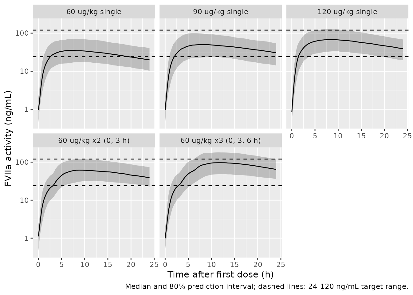
The model was then used to simulate candidate phase III regimens (Table 2, Figure 2) against a target of 24 ng/mL.
Population
46 adult males with haemophilia A or B, with or without inhibitors,
from three trials (NCT01439971, NCT04072237, NCT03407651), contributing
1225 observations (Methods “Study design and patients”, Table 1). Median
body weight 75 kg (10th-90th percentile 60-94 kg; range 43-120 kg);
median age 32 years (10th-90th percentile 23-52 years; range 18-62
years). Doses: single i.v. 4.5-30 ug/kg; single s.c. 30-120 ug/kg; 60
ug/kg s.c. two or three times 3 h apart; and daily s.c. 30 ug/kg
(escalated to 60 ug/kg on breakthrough bleeding) for 50 days. Race and
region were not reported. The same information is in the model’s
population metadata.
Source trace
| Element | Value | Source |
|---|---|---|
| Structure: 2-cmt, zero-order into depot then first-order ka | – | Results “Model development” final paragraph; Data S1
$DES
|
| Baseline added to drug concentration | IPRED = BASE + A(2)/Vc | Methods “Model building”; Data S1 $ERROR
|
| Allometry, reference 70 kg | CL, Q: 0.75; Vc, Vp: 1 | Methods “Model building”; Data S1 $PK
|
lcl |
1085 mL/h | Table S1 |
lvc |
3393 mL | Table S1 |
lvp |
619 mL | Table S1 |
lq |
213 mL/h | Table S1 |
lrbase |
0.96 ng/mL | Table S1 |
lka |
0.05 1/h | Table S1 |
logitfdepot |
logit(0.26) | Table S1; Data S1 PHI = LOG(TVF1/(1-TVF1))
|
ld1 |
0.875 h | Table S1 |
etalcl, etalvc
|
28%, 26%, correlation 0.92 | Table S1 |
etalrbase |
56% | Table S1 |
etalogitfdepot |
54% (logit scale) | Table S1 |
etalka |
30% | Table S1 |
etaiov_ld1_* |
61% | Table S1; Data S1 IOV block |
etaiov_logitfdepot_* |
21% (logit scale) | Table S1; Data S1 IOV block |
etaiov_lvc_* |
45% | Table S1; Data S1 IOV block |
propSd |
29% | Table S1; Data S1 Y = IPRED*EXP(EPS(1))
|
Virtual cohort and simulation
Faraj 2022 simulated 1000 subjects per regimen with body weight drawn
from a truncated normal distribution (bounds 40-105 kg) using the mean
and SD of the analysis data set. The mean and SD are not printed; they
are approximated here from the median (75 kg) and 10th-90th percentiles
(60-94 kg) as mean 76 kg, SD 13.3 kg. Each arm uses 200 subjects.
Subcutaneous doses go to the depot compartment with
rate = -2 so that the modelled zero-order duration D1
applies.
All simulated subjects take OCC = 2, i.e. one
subcutaneous occasion with its IOV draw. The paper does not say whether
its simulations included IOV; with IOV the simulated Tmax 80% interval
matches Table 2 (5.3-11.1 h for a single dose), while without IOV it is
about half as wide, so IOV is kept.
rxode2::rxSetSeed(20221216)
set.seed(20221216)
n_per_arm <- 200

draw_wt <- function(n) {
  x <- rnorm(5 * n, mean = 76, sd = 13.3)
  x[x >= 40 & x <= 105][seq_len(n)]
}

regimens <- tibble::tribble(
  ~treatment,             ~dose, ~times,
  "60 ug/kg single",      60,    list(0),
  "90 ug/kg single",      90,    list(0),
  "120 ug/kg single",     120,   list(0),
  "60 ug/kg x2 (0, 3 h)", 60,    list(c(0, 3)),
  "60 ug/kg x3 (0, 3, 6 h)", 60, list(c(0, 3, 6))
)

obs_times <- sort(unique(c(seq(0, 24, by = 0.25))))

make_arm <- function(k) {
  r <- regimens[k, ]
  wt <- draw_wt(n_per_arm)
  ids <- (k - 1) * n_per_arm + seq_len(n_per_arm)
  dose_times <- r$times[[1]][[1]]
  doses <- expand.grid(i = seq_len(n_per_arm), time = dose_times)
  doses <- data.frame(
    id = ids[doses$i], time = doses$time, evid = 1L,
    amt = r$dose * wt[doses$i], cmt = "depot", rate = -2,
    WT = wt[doses$i]
  )
  obs <- expand.grid(i = seq_len(n_per_arm), time = obs_times)
  obs <- data.frame(
    id = ids[obs$i], time = obs$time, evid = 0L,
    amt = 0, cmt = "central", rate = 0,
    WT = wt[obs$i]
  )
  out <- rbind(doses, obs)
  out$OCC <- 2L
  out$treatment <- r$treatment
  out
}

events <- do.call(rbind, lapply(seq_len(nrow(regimens)), make_arm))
events <- events[order(events$id, events$time, -events$evid), ]
mod <- readModelDb("Faraj_2022_marzeptacogAlfa")
sim <- rxode2::rxSolve(
  mod, events,
  keep = c("treatment", "WT"),
  returnType = "data.frame"
)
#> ℹ parameter labels from comments will be replaced by 'label()'
#> Warning: some etas defaulted to non-mu referenced, possible parsing error: etaiov_ld1_2, etaiov_ld1_3, etaiov_ld1_4, etaiov_ld1_5, etaiov_ld1_6, etaiov_ld1_7, etaiov_ld1_8, etaiov_ld1_9, etaiov_logitfdepot_2, etaiov_logitfdepot_3, etaiov_logitfdepot_4, etaiov_logitfdepot_5, etaiov_logitfdepot_6, etaiov_logitfdepot_7, etaiov_logitfdepot_8, etaiov_logitfdepot_9, etaiov_lvc_2, etaiov_lvc_3, etaiov_lvc_4, etaiov_lvc_5, etaiov_lvc_6, etaiov_lvc_7, etaiov_lvc_8, etaiov_lvc_9
#> as a work-around try putting the mu-referenced expression on a simple line
sim <- sim |>
  mutate(treatment = factor(treatment, levels = regimens$treatment))
stopifnot(!anyNA(sim$Cc))
Cc is the individual prediction without residual error
and, like the paper’s predictions, includes the endogenous FVIIa
baseline.
Concentration-time profiles
sim |>
  group_by(treatment, time) |>
  summarise(
    med = median(Cc), lo = quantile(Cc, 0.1), hi = quantile(Cc, 0.9),
    .groups = "drop"
  ) |>
  ggplot(aes(time, med)) +
  geom_ribbon(aes(ymin = lo, ymax = hi), alpha = 0.25) +
  geom_line() +
  geom_hline(yintercept = c(24, 120), linetype = "dashed") +
  facet_wrap(~treatment) +
  scale_y_log10() +
  labs(
    x = "Time after first dose (h)", y = "FVIIa activity (ng/mL)",
    caption = "Median and 80% prediction interval; dashed lines: 24-120 ng/mL target range."
  )
Percentage of the population above target (Figure 2)
above <- sim |>
  group_by(treatment, time) |>
  summarise(pct = 100 * mean(Cc >= 24), .groups = "drop")

ggplot(above, aes(time, pct, colour = treatment)) +
  geom_line() +
  geom_hline(yintercept = 90, linetype = "dashed") +
  labs(
    x = "Time after first dose (h)", y = "Population above 24 ng/mL (%)",
    colour = NULL,
    caption = "Replicates Figure 2 of Faraj 2022."
  )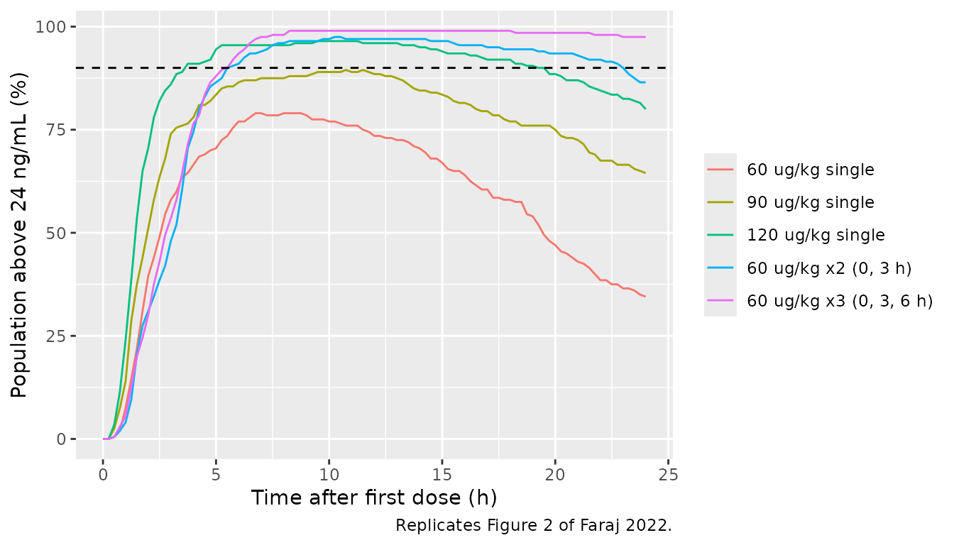
The paper reports the percentages at selected times in Results “Clinical trial simulations” and the Discussion.
ref_above <- tibble::tribble(
  ~treatment,              ~time, ~paper,
  "60 ug/kg single",       3,     51,
  "90 ug/kg single",       3,     74,
  "120 ug/kg single",      3,     86,
  "60 ug/kg single",       6,     70,
  "90 ug/kg single",       6,     87,
  "120 ug/kg single",      6,     94,
  "60 ug/kg single",       24,    33,
  "90 ug/kg single",       24,    63,
  "120 ug/kg single",      24,    78,
  "60 ug/kg x2 (0, 3 h)",  6,     90,
  "60 ug/kg x2 (0, 3 h)",  24,    81,
  "60 ug/kg x3 (0, 3, 6 h)", 9,   96
)
cmp_above <- ref_above |>
  left_join(above |> mutate(treatment = as.character(treatment)),
            by = c("treatment", "time")) |>
  mutate(diff = pct - paper)
cmp_above |>
  dplyr::rename(
    Regimen = treatment, "Time (h)" = time, "Paper (%)" = paper,
    "Simulated (%)" = pct, "Difference (points)" = diff
  ) |>
knitr::kable(digits = 0)| Regimen | Time (h) | Paper (%) | Simulated (%) | Difference (points) |
|---|---|---|---|---|
| 60 ug/kg single | 3 | 51 | 58 | 7 |
| 90 ug/kg single | 3 | 74 | 74 | 0 |
| 120 ug/kg single | 3 | 86 | 86 | 0 |
| 60 ug/kg single | 6 | 70 | 77 | 7 |
| 90 ug/kg single | 6 | 87 | 86 | 0 |
| 120 ug/kg single | 6 | 94 | 96 | 2 |
| 60 ug/kg single | 24 | 33 | 34 | 2 |
| 90 ug/kg single | 24 | 63 | 64 | 2 |
| 120 ug/kg single | 24 | 78 | 80 | 2 |
| 60 ug/kg x2 (0, 3 h) | 6 | 90 | 91 | 1 |
| 60 ug/kg x2 (0, 3 h) | 24 | 81 | 86 | 6 |
| 60 ug/kg x3 (0, 3, 6 h) | 9 | 96 | 99 | 3 |
The simulated percentages agree with the paper within a few points. With 200 subjects per arm the binomial standard error is up to 3.5 points, so differences of 5-7 points at a single time point are within sampling noise.
NCA (PKNCA) and comparison with Table 2
Table 2 reports the median and 80% prediction interval of Cmax, Tmax,
Cmin and AUC over 0-24 h. After the subcutaneous doses the concentration
rises until Tmax and then declines, so the paper’s Cmin over 24 h is the
concentration at 24 h; it is compared with PKNCA’s
clast.obs (last observation, at 24 h). The 0-24 h minimum
including the pre-dose time point would be the endogenous baseline
instead.
conc <- sim |>
  dplyr::filter(!is.na(Cc)) |>
  select(id, time, Cc, treatment)
dose <- events |>
  dplyr::filter(evid == 1) |>
  select(id, time, amt, treatment) |>
  mutate(treatment = factor(treatment, levels = regimens$treatment))

conc_obj <- PKNCA::PKNCAconc(conc, Cc ~ time | treatment + id)
dose_obj <- PKNCA::PKNCAdose(dose, amt ~ time | treatment + id)
intervals <- data.frame(
  start = 0, end = 24,
  cmax = TRUE, tmax = TRUE, clast.obs = TRUE, auclast = TRUE
)
nca <- PKNCA::pk.nca(PKNCA::PKNCAdata(conc_obj, dose_obj, intervals = intervals))
reference <- tibble::tribble(
  ~treatment,                ~cmax, ~tmax, ~clast.obs, ~auclast,
  "60 ug/kg single",         34.5,  7.8,   19.3,       604,
  "90 ug/kg single",         51.1,  7.8,   28.3,       905.3,
  "120 ug/kg single",        67.7,  7.8,   37.4,       1207.1,
  "60 ug/kg x2 (0, 3 h)",    68.7,  9.5,   40.4,       1166,
  "60 ug/kg x3 (0, 3, 6 h)", 106.1, 11.6,  66.7,       1715
)
tbl <- nlmixr2lib::ncaComparisonTable(
  simulated = nca,
  reference = reference,
  by = "treatment",
  units = c(cmax = "ng/mL", tmax = "h", clast.obs = "ng/mL", auclast = "h*ng/mL")
)
knitr::kable(tbl)| NCA parameter | treatment | Reference | Simulated | % diff |
|---|---|---|---|---|
| Cmax (ng/mL) | 60 ug/kg single | 34.5 | 35.4 | +2.5% |
| Cmax (ng/mL) | 90 ug/kg single | 51.1 | 50.1 | -2.1% |
| Cmax (ng/mL) | 120 ug/kg single | 67.7 | 68.9 | +1.8% |
| Cmax (ng/mL) | 60 ug/kg x2 (0, 3 h) | 68.7 | 62.7 | -8.8% |
| Cmax (ng/mL) | 60 ug/kg x3 (0, 3, 6 h) | 106 | 97.2 | -8.4% |
| Tmax (h) | 60 ug/kg single | 7.8 | 7.5 | -3.8% |
| Tmax (h) | 90 ug/kg single | 7.8 | 8 | +2.6% |
| Tmax (h) | 120 ug/kg single | 7.8 | 8 | +2.6% |
| Tmax (h) | 60 ug/kg x2 (0, 3 h) | 9.5 | 9.5 | +0.0% |
| Tmax (h) | 60 ug/kg x3 (0, 3, 6 h) | 11.6 | 11.8 | +1.3% |
| Clast (ng/mL) | 60 ug/kg single | 19.3 | 19.8 | +2.7% |
| Clast (ng/mL) | 90 ug/kg single | 28.3 | 30.6 | +8.1% |
| Clast (ng/mL) | 120 ug/kg single | 37.4 | 38.8 | +3.8% |
| Clast (ng/mL) | 60 ug/kg x2 (0, 3 h) | 40.4 | 39.1 | -3.3% |
| Clast (ng/mL) | 60 ug/kg x3 (0, 3, 6 h) | 66.7 | 64.2 | -3.7% |
| AUClast (h*ng/mL) | 60 ug/kg single | 604 | 659 | +9.1% |
| AUClast (h*ng/mL) | 90 ug/kg single | 905 | 936 | +3.4% |
| AUClast (h*ng/mL) | 120 ug/kg single | 1210 | 1260 | +4.7% |
| AUClast (h*ng/mL) | 60 ug/kg x2 (0, 3 h) | 1170 | 1120 | -3.9% |
| AUClast (h*ng/mL) | 60 ug/kg x3 (0, 3, 6 h) | 1720 | 1690 | -1.6% |
pct <- as.numeric(gsub("[^0-9.-]", "", tbl[["% diff"]]))
stopifnot(!anyNA(pct))
# Medians of 200 subjects; a mis-transcribed F, ka, CL or volume moves the
# whole distribution by tens of percent.
stopifnot(
  abs(median(pct)) < 7,
  quantile(abs(pct), 0.9) < 15
)
All simulated medians are within 10% of Table 2. The two repeated-dose Cmax rows run about 8% below the paper; Tmax, the 24 h concentration and AUC0-24 for the same regimens agree within 4%.
The 80% prediction intervals are compared for the single 60 ug/kg dose, where Table 2 prints Cmax 17.6-68.5 ng/mL, Tmax 5.3-11.1 h and AUC0-24 310-1190 h*ng/mL.
nca$result |>
  dplyr::filter(treatment == "60 ug/kg single",
                PPTESTCD %in% c("cmax", "tmax", "clast.obs", "auclast")) |>
  group_by(PPTESTCD) |>
  summarise(
    median = median(PPORRES), p10 = quantile(PPORRES, 0.1),
    p90 = quantile(PPORRES, 0.9), .groups = "drop"
  ) |>
  dplyr::rename(Parameter = PPTESTCD, Median = median, "10th pct" = p10, "90th pct" = p90) |>
knitr::kable(digits = 1)| Parameter | Median | 10th pct | 90th pct |
|---|---|---|---|
| auclast | 659.2 | 338.4 | 1306.0 |
| clast.obs | 19.8 | 10.3 | 40.6 |
| cmax | 35.4 | 17.6 | 72.9 |
| tmax | 7.5 | 5.2 | 11.0 |
Intravenous dosing
A typical-value profile after the 18 ug/kg i.v. dose used in two of the trials, beside the 60 ug/kg subcutaneous dose, for a 70 kg subject. The subcutaneous profile is absorption-limited (ka = 0.05 1/h is well below the elimination rate constant CL/Vc = 0.32 1/h).
typ_ev <- rbind(
  data.frame(id = 1L, time = 0, evid = 1L, amt = 18 * 70, cmt = "central", rate = 0),
  data.frame(id = 1L, time = seq(0, 48, by = 0.25), evid = 0L, amt = 0, cmt = "central", rate = 0),
  data.frame(id = 2L, time = 0, evid = 1L, amt = 60 * 70, cmt = "depot", rate = -2),
  data.frame(id = 2L, time = seq(0, 48, by = 0.25), evid = 0L, amt = 0, cmt = "central", rate = 0)
)
typ_ev$WT <- 70
typ_ev$OCC <- 1L
typ <- rxode2::rxSolve(rxode2::zeroRe(mod), typ_ev, returnType = "data.frame") |>
  mutate(route = ifelse(id == 1, "18 ug/kg i.v.", "60 ug/kg s.c."))
#> ℹ parameter labels from comments will be replaced by 'label()'
#> Warning: some etas defaulted to non-mu referenced, possible parsing error: etaiov_ld1_2, etaiov_ld1_3, etaiov_ld1_4, etaiov_ld1_5, etaiov_ld1_6, etaiov_ld1_7, etaiov_ld1_8, etaiov_ld1_9, etaiov_logitfdepot_2, etaiov_logitfdepot_3, etaiov_logitfdepot_4, etaiov_logitfdepot_5, etaiov_logitfdepot_6, etaiov_logitfdepot_7, etaiov_logitfdepot_8, etaiov_logitfdepot_9, etaiov_lvc_2, etaiov_lvc_3, etaiov_lvc_4, etaiov_lvc_5, etaiov_lvc_6, etaiov_lvc_7, etaiov_lvc_8, etaiov_lvc_9
#> as a work-around try putting the mu-referenced expression on a simple line
#> ℹ omega/sigma items treated as zero: 'etalcl', 'etalvc', 'etalrbase', 'etalogitfdepot', 'etalka', 'etaiov_ld1_2', 'etaiov_ld1_3', 'etaiov_ld1_4', 'etaiov_ld1_5', 'etaiov_ld1_6', 'etaiov_ld1_7', 'etaiov_ld1_8', 'etaiov_ld1_9', 'etaiov_logitfdepot_2', 'etaiov_logitfdepot_3', 'etaiov_logitfdepot_4', 'etaiov_logitfdepot_5', 'etaiov_logitfdepot_6', 'etaiov_logitfdepot_7', 'etaiov_logitfdepot_8', 'etaiov_logitfdepot_9', 'etaiov_lvc_2', 'etaiov_lvc_3', 'etaiov_lvc_4', 'etaiov_lvc_5', 'etaiov_lvc_6', 'etaiov_lvc_7', 'etaiov_lvc_8', 'etaiov_lvc_9'
#> Warning: multi-subject simulation without without 'omega'
stopifnot(!anyNA(typ$Cc))
ggplot(typ, aes(time, Cc, colour = route)) +
  geom_line() +
  scale_y_log10() +
  labs(x = "Time (h)", y = "FVIIa activity (ng/mL)", colour = NULL)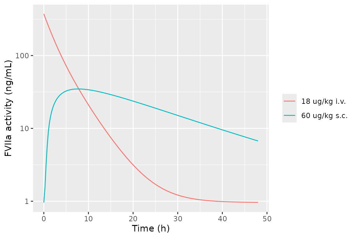
Assumptions and deviations
- Random-effect scale. Table S1 prints all random effects as percentages. They are read as 100 x the SD of the eta, so each variance is (value/100)^2. This is the only reading available for the logit-scale F etas, whose percentages cannot be log-normal CVs; for the log-normal parameters the difference from the log-normal CV conversion is small (for example 0.314 vs 0.272 for the 56% baseline IIV).
- CL-Vc correlation. Table S1 “Covariance between CL and V (%)” = 92 is read as a correlation of 0.92 (covariance 0.92 x 0.28 x 0.26 = 0.0670).
-
Initial versus final estimates. The
$THETAand$OMEGAvalues in Data S1 are initial estimates (for example CL 1300 mL/h, Vp 988 mL) and differ from the final values in Table S1, which are used here. Data S1 is used only for the model structure. - Fixed-to-zero terms omitted. Data S1 carries an absorption lag time fixed at 0 and IIV on Vp and D1 fixed at 0; these are left out. Q and Vp have no IIV.
-
Occasions. Data S1 indexes the IOV on the data
column REGI: REGI = 1 has no IOV, and REGI = 2-9 each have their own IOV
eta with a shared variance. The model’s
OCCcolumn takes the REGI value. The paper does not define REGI beyond describing IOV for subcutaneous data obtained on more than one occasion per subject. UseOCC = 1for no IOV, or 2-9 for separate occasions. - Simulation cohort. The paper simulated 1000 subjects per regimen with weights from a truncated normal distribution using the data-set mean and SD, which are not printed; this vignette uses 200 per regimen with mean 76 kg and SD 13.3 kg, approximated from the printed median and 10th-90th percentiles. Whether the paper’s simulations included IOV is not stated; including it reproduces the Table 2 Tmax interval.
-
Age. Age on ka was statistically significant but
not clinically relevant and was not retained in the final model; no
coefficient is printed, so it is recorded only in
covariatesDataExcluded. -
Endogenous baseline.
Ccincludes the endogenous FVIIa baseline (typical 0.96 ng/mL). To get the MarzAA contribution alone, subtractrbaseor setlrbaseto a very small value.