Enrofloxacin and ciprofloxacin PBPK in rainbow trout (Yang 2020)
Source:vignettes/articles/Yang_2020_enrofloxacin_rainbowTrout_pbpk.Rmd
Yang_2020_enrofloxacin_rainbowTrout_pbpk.RmdModel and source
- Citation: Yang F, Yang F, Wang D, Zhang C-S, Wang H, Song Z-W, Shao H-T, Zhang M, Yu M-L, Zheng Y. Development and application of a water temperature related physiologically based pharmacokinetic model for enrofloxacin and its metabolite ciprofloxacin in rainbow trout. Front Vet Sci. 2020;7:608348. doi:10.3389/fvets.2020.608348. Equations transcribed from the acslXtreme code in Supplementary Material section 1 (Data Sheet 1); parameter values from Tables 3-4 and the same code; Monte Carlo distributions from Supplementary Table S1.
- Article: https://doi.org/10.3389/fvets.2020.608348
- Supplementary Material (Data Sheet 1): the complete acslXtreme model code, the M-file used to compute withdrawal intervals, and Supplementary Tables S1-S3 (Monte Carlo distributions and sensitivity coefficients).
Enrofloxacin (ENR) is a veterinary fluoroquinolone used in aquaculture, and ciprofloxacin (CIP) is its main metabolite. The marker residue for ENR in fish is the sum of ENR and CIP, with a maximum residue limit (MRL) of 100 ug/kg in muscle plus skin. Fish are heterothermic, so their drug disposition depends on the water temperature. Yang and colleagues built a flow-limited whole-body PBPK model for ENR and CIP in rainbow trout in which the water temperature sets the cardiac output. They then used it to predict withdrawal intervals at 5, 10 and 16 degC.
Structure
-
ENR sub-model: stomach contents, intestinal
contents (
depot), gill, gut, liver, kidney, muscle, skin, rest of body, venous and arterial blood, plus the culture water. All cardiac output passes from venous blood through the gill to arterial blood. Liver outflow is the hepatic-artery plus gut flow. -
CIP sub-model: gill, liver, kidney, muscle, skin,
rest of body, venous and arterial blood. There is no CIP gut
compartment. CIP is formed in the liver at
Kf * A_liver, converted from mass of ENR to mass of CIP by molecular weight, and cleared renally. -
Three routes:
- Oral: the dose enters the stomach. Gastric emptying moves it to the intestinal contents, from which ENR is absorbed into the liver or lost in the faeces.
- Intravenous: the dose enters venous blood.
- Immersion bath: the bath drug is infused into the water compartment and taken up across the gill into venous blood.
-
Temperature:
CO (mL/min/kg) = 3.95 * Temp - 12.9. Every blood flow is a fixed fraction of CO. - Units: doses in mg, time in h, concentrations in ug/mL (plasma and serum) or ug/g (tissue).
The model file encodes the supplementary acslXtreme code rather than the simplified equations of Table 2 (see Errata).
mod_fn <- readModelDb("Yang_2020_enrofloxacin_rainbowTrout_pbpk")
ui <- rxode2::rxode2(mod_fn)
#> ℹ parameter labels from comments will be replaced by 'label()'
# Typical-value (deterministic) model: all Monte Carlo etas at zero.
mod0 <- rxode2::zeroRe(ui)
#> Warning: No sigma parameters in the model
Population
No new animal experiment was run. Yang 2020 digitised published plasma, serum and tissue concentrations from five rainbow trout studies (Table 1):
| Source (Yang 2020 ref) | Route and dose | Mean BW | Water temp | Use |
|---|---|---|---|---|
| 37 | IV 5, 10 mg/kg; PO 5, 10, 50 mg/kg | 100 g | 10, 15 degC | IV: optimise; PO: validate (Figure 3) |
| 3 | PO 10 mg/kg; IV 10 mg/kg | 150 g | 10, 16 degC | PO: optimise; IV: validate (Figure 2) |
| 38 | Bath 20 ppm 2.5 h, 100 ppm 0.5 h; PO 10 mg/kg | 204 g | 16.3 degC | Bath 100 ppm: optimise; others: validate (Figures 4, 7) |
| 13 | PO 10 mg/kg | 450 g | 17 degC | Optimise CIP parameters |
| 39 | PO 30 mg/kg | 50 g | 5, 10, 15 degC | Validate (Figures 5, 6) |
The unknown parameters were optimised one route at a time by Nelder-Mead in acslXtreme (Table 4). The fitted model was then used in a 500-iteration Monte Carlo analysis to predict withdrawal intervals (Table 6, Figure 8).
Source trace
| Quantity | Value | Source |
|---|---|---|
| Model equations | – | Supplementary acslXtreme code, DERIVATIVE section |
| Cardiac output |
CO = 3.95 * Temp - 12.9 mL/min/kg |
Materials and Methods; SI code |
| Volume fractions of BW (gill, liver, kidney, muscle, skin, gut, arterial, venous) | 0.039, 0.0126, 0.00841, 0.66, 0.1, 0.0852, 0.015, 0.059 | Table 3; SI code |
| Rest-of-body volume fraction | complement = 0.02079 | Table 3; SI code Vcr
|
| Blood-flow fractions of CO (liver, kidney, muscle, skin, gut) | 0.029, 0.056, 0.6, 0.053, 0.1539 | Table 3; SI code |
| Rest-of-body flow fraction | complement = 0.1081 | Table 3; SI code Qcr
|
Haematocrit pcv; serum parameter pre
|
0.304; 0.555 | Model Parameterization text; SI code |
| ENR partition coefficients (gill, liver, kidney, muscle, skin, gut, rest) | 3.46, 4.9, 11.53, 2.83, 7.38, 4.88, 0.13 | Table 3; SI code |
| CIP partition coefficients (gill, liver, kidney, muscle, skin, rest) | 2.45, 3.67, 8.2, 1.6, 0.718, 0.15 | Table 3; SI code |
Kst, KaPO, Kguc
|
0.175, 0.052, 0.605 /h | Table 4 step 2; SI code |
F |
0.6613 | Materials and Methods; SI code; Table S1 |
KaIB, Kgw, Kde
|
1.103, 0.061, 12003.31 /h | Table 4 step 3; SI code |
Kf |
0.0725 /h | Table 4 step 1; SI code |
Clre, Clmre
|
0.058, 116.14 L/h/kg | Table 4 steps 1 and 4; SI code |
Vwater |
40 L | SI code |
| Molecular weights ENR, CIP | 359.4, 331.347 g/mol | SI code |
| Monte Carlo distributions | normal, mean +/- 1 SD truncation | Monte Carlo Analysis text; Table S1 |
Two derived constants confirm the transcription. The rest-of-body fractions are computed as complements, exactly as in the code. They must reproduce the 0.02079 and 0.1081 that Table 3 prints:
fvol <- c(gill = 0.039, kidney = 0.00841, muscle = 0.66, skin = 0.1, gut = 0.0852,
          liver = 0.0126, venous = 0.059, arterial = 0.015)
fq <- c(kidney = 0.056, muscle = 0.6, skin = 0.053, liver = 0.029, gut = 0.1539)
c(fvol_remainder = 1 - sum(fvol), fq_remainder = 1 - sum(fq))
#> fvol_remainder   fq_remainder
#>        0.02079        0.10810
stopifnot(
  abs((1 - sum(fvol)) - 0.02079) < 1e-9,
  abs((1 - sum(fq)) - 0.1081) < 1e-9
)
Simulation helpers
The helpers below build event tables with named compartments.
Observations sit on the a_venous state, and every
concentration output is returned as a column. An immersion bath is dosed
into a_water as bath concentration (ppm = mg/L) times the
40 L water volume, infused over the bath duration.
# One fish, one route. `dose_mgkg` is mg/kg for PO/IV; for a bath it is the
# bath concentration in ppm, and `bath_h` the exposure time.
make_events <- function(route, dose_mgkg, wt, times, bath_h = NA_real_,
                        n_doses = 1L, tau = 24, vwater = 40) {
  dose_times <- (seq_len(n_doses) - 1) * tau
  if (route == "PO") {
    doses <- data.frame(time = dose_times, amt = dose_mgkg * wt, rate = 0,
                        cmt = "stomach")
  } else if (route == "IV") {
    doses <- data.frame(time = dose_times, amt = dose_mgkg * wt, rate = 0,
                        cmt = "a_venous")
  } else {
    amt <- dose_mgkg * vwater
    doses <- data.frame(time = dose_times, amt = amt, rate = amt / bath_h,
                        cmt = "a_water")
  }
  doses$evid <- 1L
  obs <- data.frame(time = times, amt = 0, rate = 0, cmt = "a_venous", evid = 0L)
  dplyr::bind_rows(doses, obs) |>
    dplyr::arrange(time, dplyr::desc(evid)) |>
    dplyr::mutate(id = 1L, WT = wt)
}

solve_typical <- function(events, temp) {
  events$BODYTEMP <- temp
  as.data.frame(rxode2::rxSolve(mod0, events, returnType = "data.frame"))
}
Replicate published figures
Figures 4-7: oral and immersion-bath validation
Figures 4 to 7 of Yang 2020 overlay the model prediction on the
digitised literature data. The typical-value model below regenerates
each predicted curve. Checkpoints were read by eye by the maintainers
from each figure’s predicted curve, and the model must fall within a
factor of 1.35 of each. The factor allows for reading a value off a log
axis. A mis-transcribed partition coefficient, flow or clearance shifts
these tissue curves by far more, because each tissue level scales with
its own P and the flows set every time course.
grid <- sort(unique(c(seq(0, 12, by = 0.25), seq(12, 120, by = 1))))
scen <- list(
  fig4 = list(route = "IB", dose = 20, bath_h = 2.5, wt = 0.204, temp = 16.3,
              label = "Figure 4: bath 20 ppm, 2.5 h, 16.3 degC"),
  fig7 = list(route = "PO", dose = 10, bath_h = NA, wt = 0.204, temp = 16.3,
              label = "Figure 7: PO 10 mg/kg, 16.3 degC"),
  fig6_5 = list(route = "PO", dose = 30, bath_h = NA, wt = 0.05, temp = 5,
                label = "Figures 5-6: PO 30 mg/kg, 5 degC"),
  fig6_10 = list(route = "PO", dose = 30, bath_h = NA, wt = 0.05, temp = 10,
                 label = "Figures 5-6: PO 30 mg/kg, 10 degC"),
  fig6_15 = list(route = "PO", dose = 30, bath_h = NA, wt = 0.05, temp = 15,
                 label = "Figures 5-6: PO 30 mg/kg, 15 degC")
)
sims <- lapply(names(scen), function(nm) {
  s <- scen[[nm]]
  ev <- make_events(s$route, s$dose, s$wt, grid, bath_h = s$bath_h)
  solve_typical(ev, s$temp) |> dplyr::mutate(scenario = nm, label = s$label)
}) |> dplyr::bind_rows()
#> ℹ omega/sigma items treated as zero: 'etafq_kidney', 'etafvol_muscle', 'etafvol_liver', 'etalkp_liver', 'etalkp_muscle', 'etalkp_muscle_cipro', 'etalfdepot', 'etalkmet_cipro'
#> ℹ omega/sigma items treated as zero: 'etafq_kidney', 'etafvol_muscle', 'etafvol_liver', 'etalkp_liver', 'etalkp_muscle', 'etalkp_muscle_cipro', 'etalfdepot', 'etalkmet_cipro'
#> ℹ omega/sigma items treated as zero: 'etafq_kidney', 'etafvol_muscle', 'etafvol_liver', 'etalkp_liver', 'etalkp_muscle', 'etalkp_muscle_cipro', 'etalfdepot', 'etalkmet_cipro'
#> ℹ omega/sigma items treated as zero: 'etafq_kidney', 'etafvol_muscle', 'etafvol_liver', 'etalkp_liver', 'etalkp_muscle', 'etalkp_muscle_cipro', 'etalfdepot', 'etalkmet_cipro'
#> ℹ omega/sigma items treated as zero: 'etafq_kidney', 'etafvol_muscle', 'etafvol_liver', 'etalkp_liver', 'etalkp_muscle', 'etalkp_muscle_cipro', 'etalfdepot', 'etalkmet_cipro'

long <- sims |>
  dplyr::select(scenario, label, time, Cc, Cliver, Ckidney, Cmuscle, Cskin,
                Cgut, Cliver_cipro) |>
  tidyr::pivot_longer(Cc:Cliver_cipro, names_to = "output", values_to = "conc")
long |>
  dplyr::filter(conc > 0, output != "Cliver_cipro") |>
  ggplot(aes(time, conc, colour = output)) +
  geom_line() +
  scale_y_log10() +
  facet_wrap(~label, ncol = 2) +
  labs(x = "Time (h)", y = "ENR (ug/mL or ug/g)", colour = NULL,
       title = "Replicates Figures 4, 6 and 7 of Yang 2020 (predicted curves)")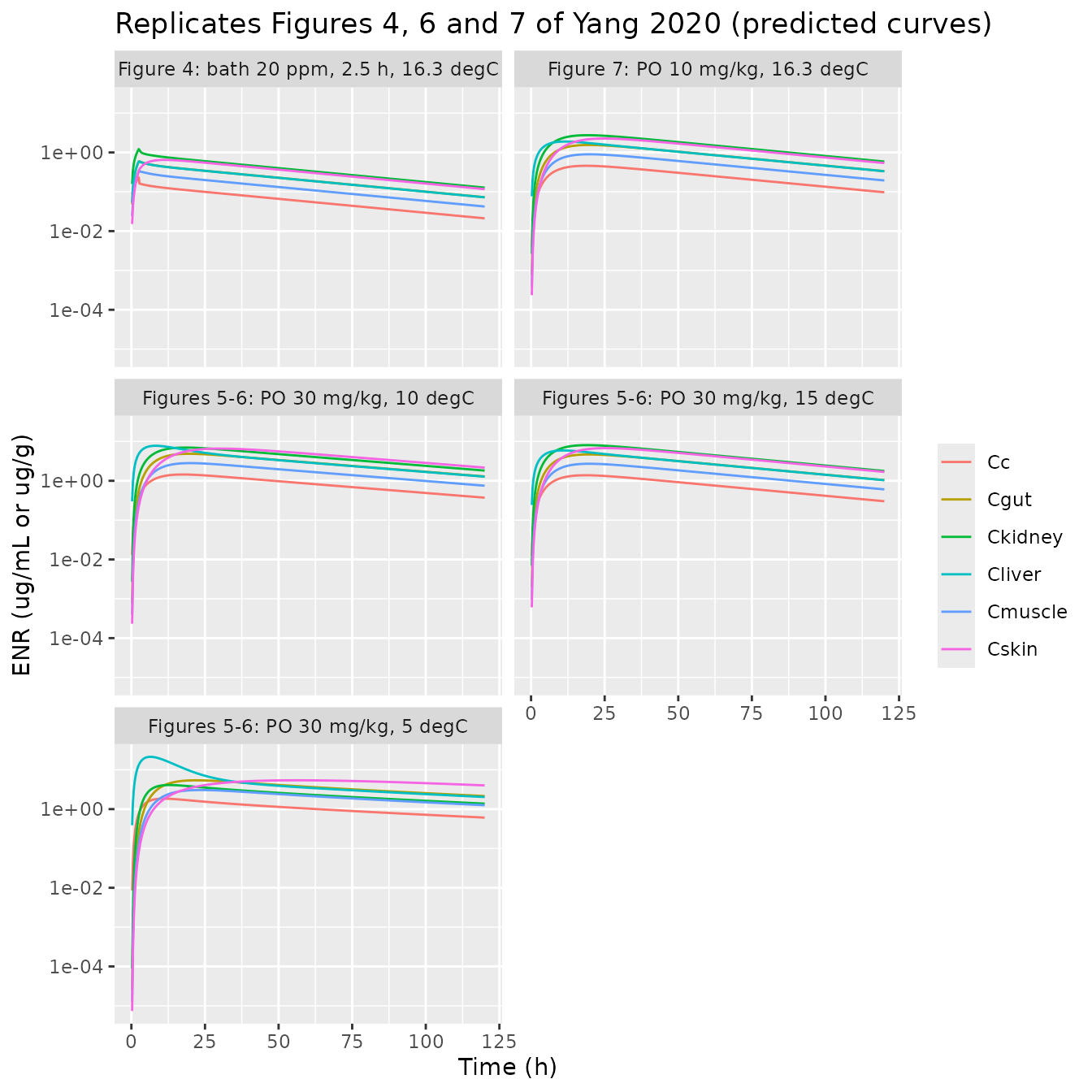
long |>
  dplyr::filter(output == "Cliver_cipro", grepl("^fig6", scenario), conc > 0) |>
  ggplot(aes(time, conc, colour = label)) +
  geom_line() +
  scale_y_log10() +
  coord_cartesian(xlim = c(0, 72)) +
  labs(x = "Time (h)", y = "CIP in liver (ug/g)", colour = NULL,
       title = "Replicates Figure 5 of Yang 2020: CIP in liver after PO 30 mg/kg")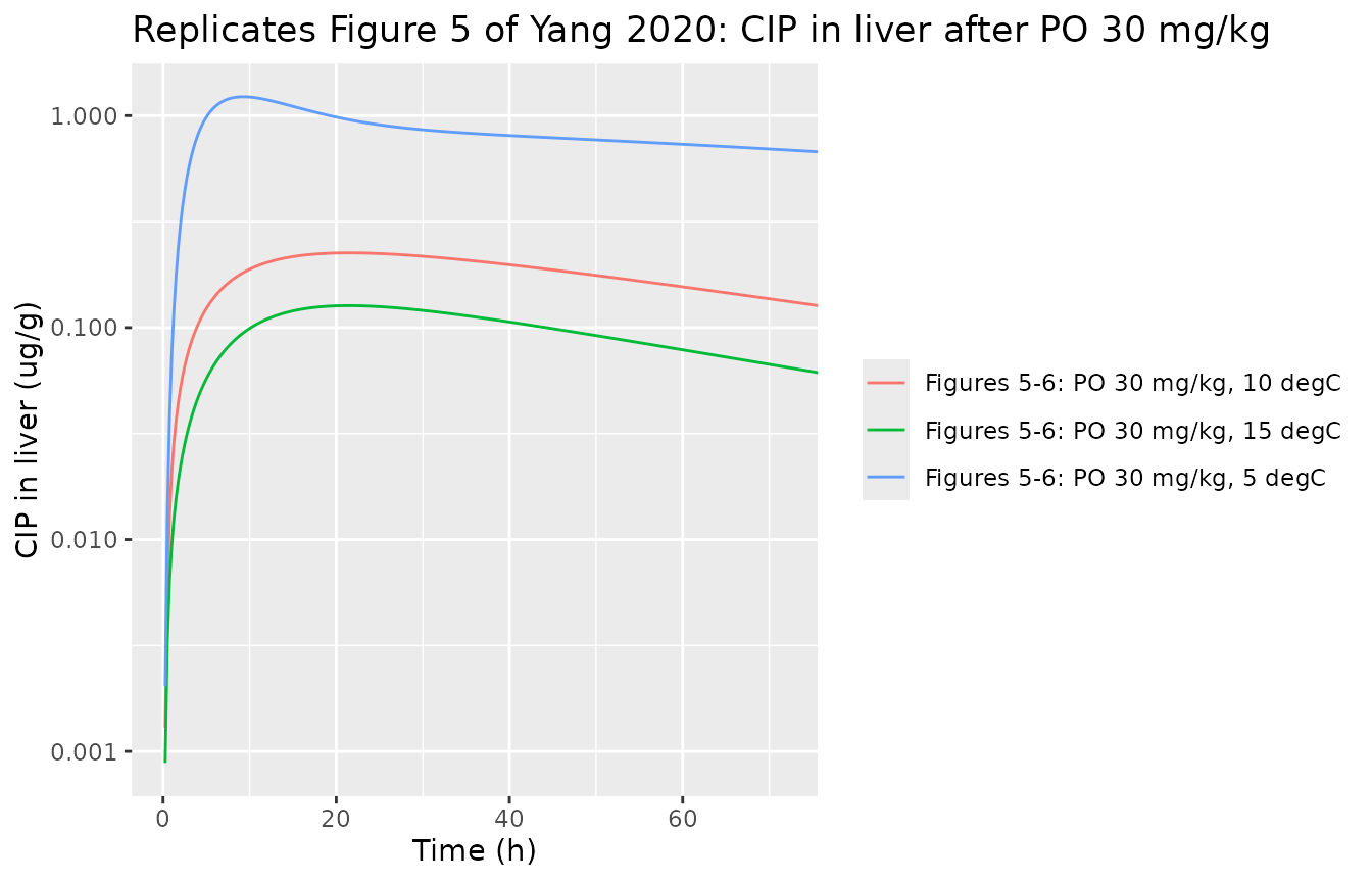
# Predicted-curve values read by eye from Yang 2020 Figures 4-7.
published <- tibble::tribble(
  ~scenario, ~output, ~time, ~published, ~source,
  "fig4", "Ckidney", 120, 0.12, "Figure 4",
  "fig4", "Cskin", 120, 0.12, "Figure 4",
  "fig4", "Cgut", 120, 0.085, "Figure 4",
  "fig4", "Cliver", 120, 0.07, "Figure 4",
  "fig4", "Cmuscle", 120, 0.04, "Figure 4",
  "fig4", "Cc", 120, 0.02, "Figure 4",
  "fig7", "Cc", 12, 0.42, "Figure 7 inset",
  "fig7", "Ckidney", 12, 2.4, "Figure 7 inset",
  "fig7", "Cliver", 12, 1.9, "Figure 7 inset",
  "fig7", "Cskin", 12, 1.5, "Figure 7 inset",
  "fig7", "Cgut", 12, 1.35, "Figure 7 inset",
  "fig7", "Cmuscle", 12, 0.8, "Figure 7 inset",
  "fig6_5", "Cc", 12, 1.8, "Figure 6A",
  "fig6_5", "Cliver", 8, 21, "Figure 6A",
  "fig6_5", "Cliver", 24, 7.5, "Figure 6A",
  "fig6_5", "Cmuscle", 24, 3.0, "Figure 6A",
  "fig6_5", "Cc", 72, 0.9, "Figure 6A",
  "fig6_10", "Cc", 24, 1.4, "Figure 6B",
  "fig6_10", "Cliver", 8, 7.8, "Figure 6B",
  "fig6_10", "Cmuscle", 24, 2.8, "Figure 6B",
  "fig6_10", "Cc", 72, 0.72, "Figure 6B",
  "fig6_15", "Cc", 24, 1.35, "Figure 6C",
  "fig6_15", "Cliver", 8, 5.8, "Figure 6C",
  "fig6_15", "Cmuscle", 24, 2.7, "Figure 6C",
  "fig6_15", "Cc", 72, 0.65, "Figure 6C",
  "fig6_5", "Cliver_cipro", 8, 1.15, "Figure 5",
  "fig6_5", "Cliver_cipro", 72, 0.62, "Figure 5",
  "fig6_10", "Cliver_cipro", 24, 0.22, "Figure 5",
  "fig6_10", "Cliver_cipro", 72, 0.153, "Figure 5",
  "fig6_15", "Cliver_cipro", 24, 0.138, "Figure 5",
  "fig6_15", "Cliver_cipro", 72, 0.083, "Figure 5"
)
chk <- published |>
  dplyr::left_join(long, by = c("scenario", "output", "time")) |>
  dplyr::mutate(ratio = conc / published)
chk |>
  dplyr::select(Figure = source, Scenario = scenario, Output = output,
                `Time (h)` = time, Published = published, Model = conc,
                `Model / published` = ratio) |>
knitr::kable(digits = 3)| Figure | Scenario | Output | Time (h) | Published | Model | Model / published |
|---|---|---|---|---|---|---|
| Figure 4 | fig4 | Ckidney | 120 | 0.120 | 0.128 | 1.063 |
| Figure 4 | fig4 | Cskin | 120 | 0.120 | 0.117 | 0.974 |
| Figure 4 | fig4 | Cgut | 120 | 0.085 | 0.073 | 0.855 |
| Figure 4 | fig4 | Cliver | 120 | 0.070 | 0.072 | 1.033 |
| Figure 4 | fig4 | Cmuscle | 120 | 0.040 | 0.042 | 1.056 |
| Figure 4 | fig4 | Cc | 120 | 0.020 | 0.021 | 1.056 |
| Figure 7 inset | fig7 | Cc | 12 | 0.420 | 0.418 | 0.995 |
| Figure 7 inset | fig7 | Ckidney | 12 | 2.400 | 2.460 | 1.025 |
| Figure 7 inset | fig7 | Cliver | 12 | 1.900 | 1.894 | 0.997 |
| Figure 7 inset | fig7 | Cskin | 12 | 1.500 | 1.534 | 1.023 |
| Figure 7 inset | fig7 | Cgut | 12 | 1.350 | 1.360 | 1.008 |
| Figure 7 inset | fig7 | Cmuscle | 12 | 0.800 | 0.783 | 0.979 |
| Figure 6A | fig6_5 | Cc | 12 | 1.800 | 1.840 | 1.022 |
| Figure 6A | fig6_5 | Cliver | 8 | 21.000 | 20.776 | 0.989 |
| Figure 6A | fig6_5 | Cliver | 24 | 7.500 | 7.409 | 0.988 |
| Figure 6A | fig6_5 | Cmuscle | 24 | 3.000 | 3.057 | 1.019 |
| Figure 6A | fig6_5 | Cc | 72 | 0.900 | 0.919 | 1.021 |
| Figure 6B | fig6_10 | Cc | 24 | 1.400 | 1.387 | 0.991 |
| Figure 6B | fig6_10 | Cliver | 8 | 7.800 | 7.767 | 0.996 |
| Figure 6B | fig6_10 | Cmuscle | 24 | 2.800 | 2.763 | 0.987 |
| Figure 6B | fig6_10 | Cc | 72 | 0.720 | 0.719 | 0.999 |
| Figure 6C | fig6_15 | Cc | 24 | 1.350 | 1.342 | 0.994 |
| Figure 6C | fig6_15 | Cliver | 8 | 5.800 | 5.721 | 0.986 |
| Figure 6C | fig6_15 | Cmuscle | 24 | 2.700 | 2.660 | 0.985 |
| Figure 6C | fig6_15 | Cc | 72 | 0.650 | 0.649 | 0.998 |
| Figure 5 | fig6_5 | Cliver_cipro | 8 | 1.150 | 1.213 | 1.055 |
| Figure 5 | fig6_5 | Cliver_cipro | 72 | 0.620 | 0.689 | 1.111 |
| Figure 5 | fig6_10 | Cliver_cipro | 24 | 0.220 | 0.224 | 1.020 |
| Figure 5 | fig6_10 | Cliver_cipro | 72 | 0.153 | 0.133 | 0.871 |
| Figure 5 | fig6_15 | Cliver_cipro | 24 | 0.138 | 0.126 | 0.914 |
| Figure 5 | fig6_15 | Cliver_cipro | 72 | 0.083 | 0.065 | 0.783 |
stopifnot(
  nrow(chk) == nrow(published),
  all(is.finite(chk$ratio)),
  all(abs(log(chk$ratio)) < log(1.35)),
  abs(median(log(chk$ratio))) < log(1.1)
)
All 31 checkpoints are within the tolerance, and the median ratio is close to 1. So the model reproduces the authors’ own predictions for the oral route at 5, 10, 15 and 16.3 degC and for the 20 ppm bath. That covers ENR in plasma and five tissues and CIP in liver. The largest gap is CIP in liver at 15 degC, where the model is about 22% below Figure 5 at 72 h.
Figures 2 and 3: IV and low-dose oral validation
Figures 2 and 3 are not reproduced by the published code, and no setting of it can reproduce Figure 3.
iv <- solve_typical(make_events("IV", 10, 0.15, c(4, 24, 48, 72, 96)), 16)
#> ℹ omega/sigma items treated as zero: 'etafq_kidney', 'etafvol_muscle', 'etafvol_liver', 'etalkp_liver', 'etalkp_muscle', 'etalkp_muscle_cipro', 'etalfdepot', 'etalkmet_cipro'
po <- lapply(c(5, 10, 50), function(d) {
  solve_typical(make_events("PO", d, 0.1, c(12, 60)), 10) |>
    dplyr::mutate(dose = d)
}) |> dplyr::bind_rows()
#> ℹ omega/sigma items treated as zero: 'etafq_kidney', 'etafvol_muscle', 'etafvol_liver', 'etalkp_liver', 'etalkp_muscle', 'etalkp_muscle_cipro', 'etalfdepot', 'etalkmet_cipro'
#> ℹ omega/sigma items treated as zero: 'etafq_kidney', 'etafvol_muscle', 'etafvol_liver', 'etalkp_liver', 'etalkp_muscle', 'etalkp_muscle_cipro', 'etalfdepot', 'etalkmet_cipro'
#> ℹ omega/sigma items treated as zero: 'etafq_kidney', 'etafvol_muscle', 'etafvol_liver', 'etalkp_liver', 'etalkp_muscle', 'etalkp_muscle_cipro', 'etalfdepot', 'etalkmet_cipro'

fig2 <- tibble::tibble(
  Figure = "2 (IV 10 mg/kg, 16 degC, plasma)",
  `Time (h)` = c(4, 24, 48, 72, 96),
  Published = c(7.9, 5.2, 3.2, 2.1, 1.2),
  Model = iv$Cc
)
fig3 <- tibble::tibble(
  Figure = paste0("3A (PO ", po$dose, " mg/kg, 10 degC, serum)"),
  `Time (h)` = po$time,
  Published = c(0.85, 0.45, 1.12, 0.63, 4.4, 2.1),
  Model = po$Cserum
)
dplyr::bind_rows(fig2, fig3) |>
  dplyr::mutate(`Model / published` = Model / Published) |>
knitr::kable(digits = 3)| Figure | Time (h) | Published | Model | Model / published |
|---|---|---|---|---|
| 2 (IV 10 mg/kg, 16 degC, plasma) | 4 | 7.90 | 4.062 | 0.514 |
| 2 (IV 10 mg/kg, 16 degC, plasma) | 24 | 5.20 | 2.751 | 0.529 |
| 2 (IV 10 mg/kg, 16 degC, plasma) | 48 | 3.20 | 1.863 | 0.582 |
| 2 (IV 10 mg/kg, 16 degC, plasma) | 72 | 2.10 | 1.262 | 0.601 |
| 2 (IV 10 mg/kg, 16 degC, plasma) | 96 | 1.20 | 0.855 | 0.713 |
| 3A (PO 5 mg/kg, 10 degC, serum) | 12 | 0.85 | 0.354 | 0.417 |
| 3A (PO 5 mg/kg, 10 degC, serum) | 60 | 0.45 | 0.221 | 0.491 |
| 3A (PO 10 mg/kg, 10 degC, serum) | 12 | 1.12 | 0.708 | 0.632 |
| 3A (PO 10 mg/kg, 10 degC, serum) | 60 | 0.63 | 0.442 | 0.702 |
| 3A (PO 50 mg/kg, 10 degC, serum) | 12 | 4.40 | 3.542 | 0.805 |
| 3A (PO 50 mg/kg, 10 degC, serum) | 60 | 2.10 | 2.211 | 1.053 |
The model is linear in dose: every process is first order. Serum at 12 h per mg/kg must therefore be the same for the 5, 10 and 50 mg/kg arms of Figure 3, and it is in the simulation. The published predicted curves give 0.170, 0.112 and 0.088 ug/mL per mg/kg: they are not dose-proportional. No set of fixed parameter values yields them, so they were not produced by the deposited code at a single parameter set.
Figure 2 is the IV validation at 16 degC. It sits about 1.9-fold above the model at 24 h, and its terminal decline (about 0.020 /h) is faster than the model’s (0.016 /h). The model’s terminal rate follows from the printed parameters: total ENR clearance over the steady-state distribution volume. It cannot be brought to Figure 2 without changing a printed value. Figures 4 to 7 match, and they exercise the same distribution and elimination parameters (all routes share them; Model Parameterization text). So the deposited code is treated as the model, and Figures 2 and 3 as figures that were generated some other way.
Mass balance
The code carries a mass-balance check (MBenr,
MBcip) that “should eventually approach zero”. Every ENR
elimination path ends either in the water (renal, faecal and branchial
loss) or in a_degraded (degradation in the water) and
a_metabolized (conversion to CIP). So the dose must equal
the sum of all ENR states at every time. CIP formed must equal CIP in
the body plus CIP excreted renally.
mb_ev <- dplyr::bind_rows(
  make_events("PO", 10, 0.05, seq(0, 240, by = 6)) |> dplyr::mutate(id = 1L),
  make_events("IV", 10, 0.05, seq(0, 240, by = 6)) |> dplyr::mutate(id = 2L),
  make_events("IB", 20, 0.05, seq(0, 240, by = 6), bath_h = 2.5) |>
    dplyr::mutate(id = 3L)
)
mb <- solve_typical(mb_ev, 10) |>
  dplyr::mutate(
    dose = c(10 * 0.05, 10 * 0.05, 20 * 40)[id],
    enr_total = a_water + a_degraded + stomach + depot + a_gill + a_gut +
      a_liver + a_metabolized + a_kidney + a_muscle + a_skin + a_remainder +
      a_venous + a_arterial,
    cip_formed = a_metabolized * 331.347 / 359.4,
    cip_total = a_liver_cipro + a_kidney_cipro + a_urine_cipro +
      a_muscle_cipro + a_skin_cipro + a_remainder_cipro + a_gill_cipro +
      a_venous_cipro + a_arterial_cipro
  )
#> ℹ omega/sigma items treated as zero: 'etafq_kidney', 'etafvol_muscle', 'etafvol_liver', 'etalkp_liver', 'etalkp_muscle', 'etalkp_muscle_cipro', 'etalfdepot', 'etalkmet_cipro'
# The bath infusion is still running before 2.5 h; check after it ends.
mb_after <- mb |> dplyr::filter(time >= 3)
c(max_enr_error = max(abs(mb_after$enr_total - mb_after$dose) / mb_after$dose),
  max_cip_error = max(abs(mb_after$cip_total - mb_after$cip_formed) /
                        pmax(mb_after$cip_formed, 1e-12)))
#> max_enr_error max_cip_error
#>  6.257106e-12  2.460445e-13
stopifnot(
  all(abs(mb_after$enr_total - mb_after$dose) / mb_after$dose < 1e-6),
  all(abs(mb_after$cip_total - mb_after$cip_formed) <= 1e-6 * mb_after$dose)
)
A mutation check shows the gate is not vacuous. If the two water-side sinks (the water compartment and the degraded amount, which together receive the renal, faecal and branchial losses) are left out of the total, the ENR total drifts away from the dose:
Withdrawal intervals
Yang 2020 defines the withdrawal interval as the time at which ENR + CIP in muscle (or skin) falls below the 0.1 ug/g MRL for good. It is taken at the 99th percentile of 500 Monte Carlo fish (M-file in the Supplementary Material; Table 6).
Typical fish
The typical fish is simulated with the code’s default body weight of 0.05 kg. Concentrations after oral dosing do not depend on body weight; after a bath they scale as 1 / body weight (see Errata). For the 7-day regimen, the interval is counted from the last dose.
# First grid time after the last MRL exceedance, in days from the last dose,
# rounded up to whole days as in Table 6.
withdrawal_days <- function(time, conc, t_last_dose, mrl = 0.1) {
  above <- which(conc > mrl)
  if (length(above) == 0L) return(0)
  i <- max(above)
  if (i == length(time)) stop("MRL not reached within the simulated horizon")
  ceiling((time[i + 1L] - t_last_dose) / 24)
}

regimens <- tibble::tribble(
  ~regimen, ~route, ~dose, ~bath_h, ~n_doses,
  "Single oral dose (10 mg/kg)", "PO", 10, NA, 1L,
  "Multiple oral dose (20 mg/kg/day x 7)", "PO", 20, NA, 7L,
  "Bath 20 ppm for 2.5 h", "IB", 20, 2.5, 1L,
  "Bath 100 ppm for 0.5 h", "IB", 100, 0.5, 1L
)
wd_grid <- seq(0, 60 * 24, by = 1)
typical_wd <- tidyr::crossing(regimens, temp = c(5, 10, 16)) |>
  dplyr::rowwise() |>
  dplyr::mutate(sim = list(solve_typical(
    make_events(route, dose, 0.05, wd_grid, bath_h = bath_h, n_doses = n_doses),
    temp
  ))) |>
  dplyr::mutate(
    muscle = withdrawal_days(sim$time, sim$Cmuscle_total, (n_doses - 1) * 24),
    skin = withdrawal_days(sim$time, sim$Cskin_total, (n_doses - 1) * 24)
  ) |>
  dplyr::ungroup() |>
  dplyr::select(regimen, temp, muscle, skin)
#> ℹ omega/sigma items treated as zero: 'etafq_kidney', 'etafvol_muscle', 'etafvol_liver', 'etalkp_liver', 'etalkp_muscle', 'etalkp_muscle_cipro', 'etalfdepot', 'etalkmet_cipro'
#> ℹ omega/sigma items treated as zero: 'etafq_kidney', 'etafvol_muscle', 'etafvol_liver', 'etalkp_liver', 'etalkp_muscle', 'etalkp_muscle_cipro', 'etalfdepot', 'etalkmet_cipro'
#> ℹ omega/sigma items treated as zero: 'etafq_kidney', 'etafvol_muscle', 'etafvol_liver', 'etalkp_liver', 'etalkp_muscle', 'etalkp_muscle_cipro', 'etalfdepot', 'etalkmet_cipro'
#> ℹ omega/sigma items treated as zero: 'etafq_kidney', 'etafvol_muscle', 'etafvol_liver', 'etalkp_liver', 'etalkp_muscle', 'etalkp_muscle_cipro', 'etalfdepot', 'etalkmet_cipro'
#> ℹ omega/sigma items treated as zero: 'etafq_kidney', 'etafvol_muscle', 'etafvol_liver', 'etalkp_liver', 'etalkp_muscle', 'etalkp_muscle_cipro', 'etalfdepot', 'etalkmet_cipro'
#> ℹ omega/sigma items treated as zero: 'etafq_kidney', 'etafvol_muscle', 'etafvol_liver', 'etalkp_liver', 'etalkp_muscle', 'etalkp_muscle_cipro', 'etalfdepot', 'etalkmet_cipro'
#> ℹ omega/sigma items treated as zero: 'etafq_kidney', 'etafvol_muscle', 'etafvol_liver', 'etalkp_liver', 'etalkp_muscle', 'etalkp_muscle_cipro', 'etalfdepot', 'etalkmet_cipro'
#> ℹ omega/sigma items treated as zero: 'etafq_kidney', 'etafvol_muscle', 'etafvol_liver', 'etalkp_liver', 'etalkp_muscle', 'etalkp_muscle_cipro', 'etalfdepot', 'etalkmet_cipro'
#> ℹ omega/sigma items treated as zero: 'etafq_kidney', 'etafvol_muscle', 'etafvol_liver', 'etalkp_liver', 'etalkp_muscle', 'etalkp_muscle_cipro', 'etalfdepot', 'etalkmet_cipro'
#> ℹ omega/sigma items treated as zero: 'etafq_kidney', 'etafvol_muscle', 'etafvol_liver', 'etalkp_liver', 'etalkp_muscle', 'etalkp_muscle_cipro', 'etalfdepot', 'etalkmet_cipro'
#> ℹ omega/sigma items treated as zero: 'etafq_kidney', 'etafvol_muscle', 'etafvol_liver', 'etalkp_liver', 'etalkp_muscle', 'etalkp_muscle_cipro', 'etalfdepot', 'etalkmet_cipro'
#> ℹ omega/sigma items treated as zero: 'etafq_kidney', 'etafvol_muscle', 'etafvol_liver', 'etalkp_liver', 'etalkp_muscle', 'etalkp_muscle_cipro', 'etalfdepot', 'etalkmet_cipro'

# Yang 2020 Table 6 (99th percentile of the Monte Carlo population, days).
table6 <- tibble::tribble(
  ~regimen, ~temp, ~muscle_t6, ~skin_t6,
  "Single oral dose (10 mg/kg)", 5, 18, 24,
  "Single oral dose (10 mg/kg)", 10, 11, 14,
  "Single oral dose (10 mg/kg)", 16, 9, 12,
  "Multiple oral dose (20 mg/kg/day x 7)", 5, 30, 36,
  "Multiple oral dose (20 mg/kg/day x 7)", 10, 17, 20,
  "Multiple oral dose (20 mg/kg/day x 7)", 16, 14, 17,
  "Bath 20 ppm for 2.5 h", 5, 16, 22,
  "Bath 20 ppm for 2.5 h", 10, 9, 12,
  "Bath 20 ppm for 2.5 h", 16, 8, 10,
  "Bath 100 ppm for 0.5 h", 5, 26, 31,
  "Bath 100 ppm for 0.5 h", 10, 15, 18,
  "Bath 100 ppm for 0.5 h", 16, 13, 15
)
wd_cmp <- typical_wd |> dplyr::left_join(table6, by = c("regimen", "temp"))
wd_cmp |>
  dplyr::select(Regimen = regimen, `Water temp (degC)` = temp,
                `Muscle, typical fish (d)` = muscle,
                `Muscle, Table 6 P99 (d)` = muscle_t6,
                `Skin, typical fish (d)` = skin,
                `Skin, Table 6 P99 (d)` = skin_t6) |>
knitr::kable()| Regimen | Water temp (degC) | Muscle, typical fish (d) | Muscle, Table 6 P99 (d) | Skin, typical fish (d) | Skin, Table 6 P99 (d) |
|---|---|---|---|---|---|
| Bath 100 ppm for 0.5 h | 5 | 22 | 26 | 28 | 31 |
| Bath 100 ppm for 0.5 h | 10 | 13 | 15 | 16 | 18 |
| Bath 100 ppm for 0.5 h | 16 | 11 | 13 | 14 | 15 |
| Bath 20 ppm for 2.5 h | 5 | 14 | 16 | 20 | 22 |
| Bath 20 ppm for 2.5 h | 10 | 8 | 9 | 11 | 12 |
| Bath 20 ppm for 2.5 h | 16 | 7 | 8 | 10 | 10 |
| Multiple oral dose (20 mg/kg/day x 7) | 5 | 25 | 30 | 31 | 36 |
| Multiple oral dose (20 mg/kg/day x 7) | 10 | 14 | 17 | 17 | 20 |
| Multiple oral dose (20 mg/kg/day x 7) | 16 | 12 | 14 | 14 | 17 |
| Single oral dose (10 mg/kg) | 5 | 14 | 18 | 20 | 24 |
| Single oral dose (10 mg/kg) | 10 | 8 | 11 | 12 | 14 |
| Single oral dose (10 mg/kg) | 16 | 7 | 9 | 10 | 12 |
stopifnot(
  nrow(wd_cmp) == 12L,
  all(wd_cmp$muscle <= wd_cmp$muscle_t6),
  all(wd_cmp$skin <= wd_cmp$skin_t6),
  all(wd_cmp$skin >= wd_cmp$muscle)
)
For every regimen and temperature, the typical fish clears below Table 6’s 99th-percentile interval, and skin takes longer than muscle, as the paper reports. The multiple-dose regimen allows a sharper check. Figure 8 plots the full Monte Carlo distribution of its withdrawal interval, and a typical fish should sit at the centre of that distribution. The medians below were read by the maintainers from the Figure 8 histograms:
fig8 <- tibble::tribble(
  ~temp, ~muscle_fig8, ~skin_fig8,
  16, 12, 14.5,
  10, 14, 17,
  5, 25.5, 31
)
f8 <- typical_wd |>
  dplyr::filter(grepl("^Multiple", regimen)) |>
  dplyr::left_join(fig8, by = "temp")
f8 |>
  dplyr::select(`Water temp (degC)` = temp, `Muscle, typical (d)` = muscle,
                `Muscle, Fig 8 median (d)` = muscle_fig8,
                `Skin, typical (d)` = skin, `Skin, Fig 8 median (d)` = skin_fig8) |>
knitr::kable()| Water temp (degC) | Muscle, typical (d) | Muscle, Fig 8 median (d) | Skin, typical (d) | Skin, Fig 8 median (d) |
|---|---|---|---|---|
| 5 | 25 | 25.5 | 31 | 31.0 |
| 10 | 14 | 14.0 | 17 | 17.0 |
| 16 | 12 | 12.0 | 14 | 14.5 |
The agreement holds only when the interval is counted from the last dose. Counted from the first dose, every value would be 6 days longer, which is outside the histograms.
Monte Carlo population
The eight Table S1 parameters carry between-fish variability in the model file. The draws below use standard-normal deviates generated in R and passed to the typical-value model as data. That keeps the cohort identical on every machine; rxode2’s own random-number streams depend on the solver thread count. Each deviate is mapped inside the model onto the Table S1 normal distribution truncated at mean +/- 1 SD. Yang 2020 also varied the water temperature within each run, but its distribution is not reported, so here it is held at 5, 10 or 16 degC. This population is therefore narrower than the authors’ one.
set.seed(20200125)
n_fish <- 200L
eta_names <- c("etafq_kidney", "etafvol_muscle", "etafvol_liver",
               "etalkp_liver", "etalkp_muscle", "etalkp_muscle_cipro",
               "etalfdepot", "etalkmet_cipro")
eta_draws <- as.data.frame(matrix(rnorm(n_fish * length(eta_names)), n_fish,
                                  dimnames = list(NULL, eta_names)))
eta_draws$id <- seq_len(n_fish)

mc_grid <- seq(0, 51 * 24, by = 4)
base_ev <- make_events("PO", 20, 0.05, mc_grid, n_doses = 7L) |> dplyr::select(-id)
mc_ev <- tidyr::crossing(id = seq_len(n_fish), base_ev) |>
  dplyr::left_join(eta_draws, by = "id") |>
  dplyr::arrange(id, time, dplyr::desc(evid))

mc_wd <- lapply(c(5, 10, 16), function(temp) {
  ev <- mc_ev
  ev$BODYTEMP <- temp
  s <- rxode2::rxSolve(mod0, ev, returnType = "data.frame")
  s <- as.data.frame(s)[, c("id", "time", "Cmuscle_total", "Cskin_total")]
  s |>
    dplyr::group_by(id) |>
    dplyr::summarise(
      muscle = withdrawal_days(time, Cmuscle_total, 6 * 24),
      skin = withdrawal_days(time, Cskin_total, 6 * 24),
      .groups = "drop"
    ) |>
    dplyr::mutate(temp = temp)
}) |> dplyr::bind_rows()
#> ℹ omega/sigma items treated as zero: 'etafq_kidney', 'etafvol_muscle', 'etafvol_liver', 'etalkp_liver', 'etalkp_muscle', 'etalkp_muscle_cipro', 'etalfdepot', 'etalkmet_cipro'
#> ℹ omega/sigma items treated as zero: 'etafq_kidney', 'etafvol_muscle', 'etafvol_liver', 'etalkp_liver', 'etalkp_muscle', 'etalkp_muscle_cipro', 'etalfdepot', 'etalkmet_cipro'
#> ℹ omega/sigma items treated as zero: 'etafq_kidney', 'etafvol_muscle', 'etafvol_liver', 'etalkp_liver', 'etalkp_muscle', 'etalkp_muscle_cipro', 'etalfdepot', 'etalkmet_cipro'

mc_sum <- mc_wd |>
  tidyr::pivot_longer(c(muscle, skin), names_to = "tissue", values_to = "days") |>
  dplyr::group_by(temp, tissue) |>
  dplyr::summarise(median = median(days),
                   p99 = unname(quantile(days, 0.99, type = 1)),
                   .groups = "drop")
mc_ref <- table6 |>
  dplyr::filter(grepl("^Multiple", regimen)) |>
  dplyr::select(temp, muscle = muscle_t6, skin = skin_t6) |>
  tidyr::pivot_longer(c(muscle, skin), names_to = "tissue", values_to = "table6_p99") |>
  dplyr::left_join(
    fig8 |> dplyr::rename(muscle = muscle_fig8, skin = skin_fig8) |>
      tidyr::pivot_longer(c(muscle, skin), names_to = "tissue",
                          values_to = "fig8_median"),
    by = c("temp", "tissue")
  )
mc_tab <- mc_sum |> dplyr::left_join(mc_ref, by = c("temp", "tissue"))
mc_tab |>
  dplyr::select(`Water temp (degC)` = temp, Tissue = tissue,
                `Simulated median (d)` = median, `Figure 8 median (d)` = fig8_median,
                `Simulated P99 (d)` = p99, `Table 6 P99 (d)` = table6_p99) |>
knitr::kable()| Water temp (degC) | Tissue | Simulated median (d) | Figure 8 median (d) | Simulated P99 (d) | Table 6 P99 (d) |
|---|---|---|---|---|---|
| 5 | muscle | 25 | 25.5 | 29 | 30 |
| 5 | skin | 31 | 31.0 | 35 | 36 |
| 10 | muscle | 14 | 14.0 | 16 | 17 |
| 10 | skin | 17 | 17.0 | 19 | 20 |
| 16 | muscle | 12 | 12.0 | 13 | 14 |
| 16 | skin | 14 | 14.5 | 16 | 17 |
stopifnot(
  all(abs(mc_tab$median - mc_tab$fig8_median) <= 1.5),
  all(mc_tab$p99 <= mc_tab$table6_p99 + 1)
)
mc_wd |>
  tidyr::pivot_longer(c(muscle, skin), names_to = "tissue", values_to = "days") |>
  ggplot(aes(days, fill = factor(temp))) +
  geom_histogram(binwidth = 1, position = "identity", alpha = 0.5) +
  facet_wrap(~tissue, ncol = 1) +
  labs(x = "Withdrawal interval after the last dose (days)",
       y = "Number of simulated fish", fill = "Water temp (degC)",
       title = "Replicates Figure 8 of Yang 2020 (20 mg/kg/day for 7 days)")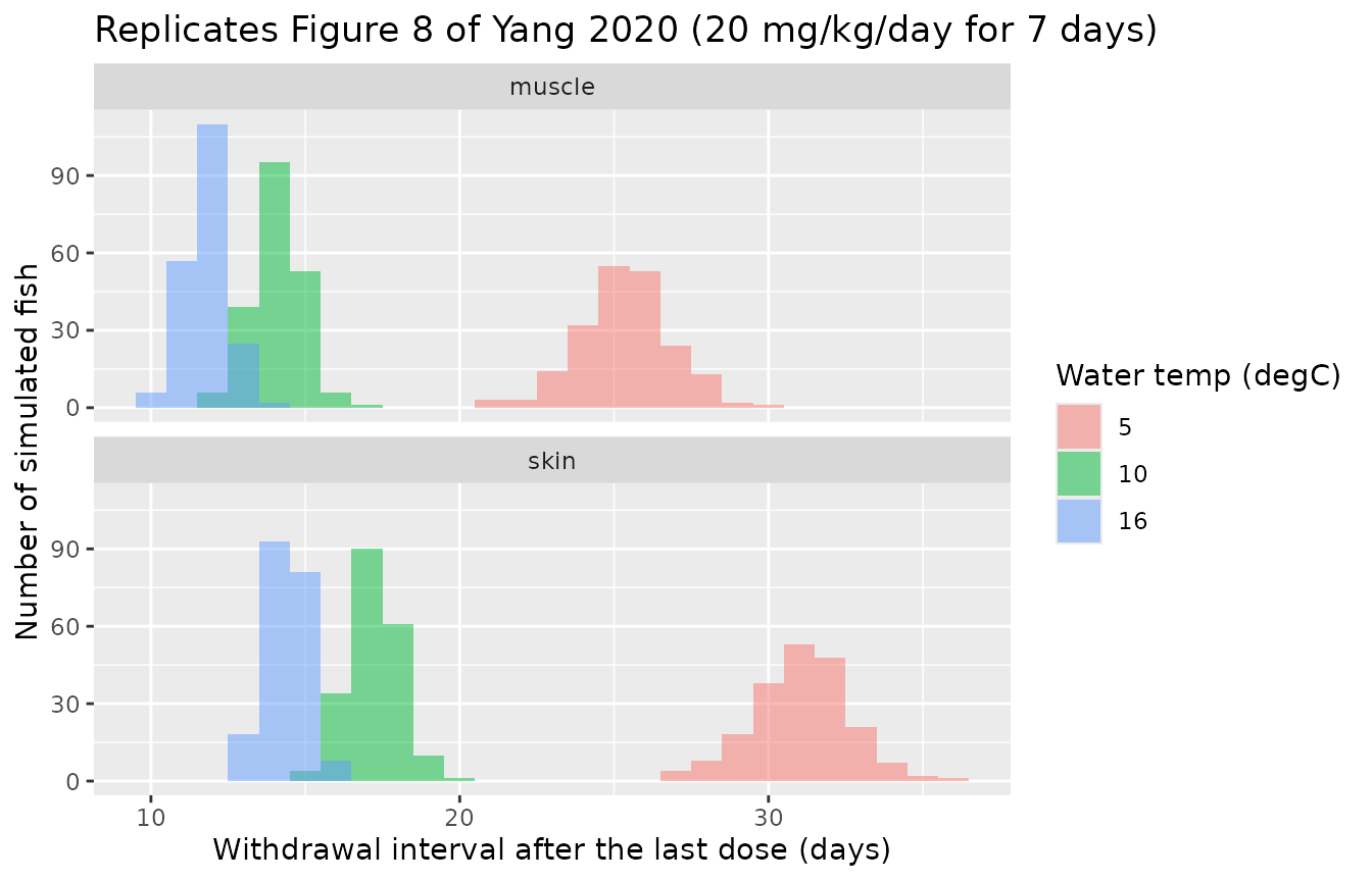
The simulated medians match Figure 8. The simulated 99th percentiles sit at or below Table 6, as expected when the water-temperature variability of the authors’ runs is left out.
PKNCA validation
Yang 2020 reports no NCA parameters, so the NCA here characterises the model rather than comparing with the paper. Two properties are asserted:
- ENR elimination slows as the water cools, because every blood flow, including renal blood flow, scales with cardiac output.
- The model is exactly dose-linear.
nca_grid <- sort(unique(c(seq(0, 24, by = 0.5), seq(24, 480, by = 4))))
nca_cases <- tibble::tribble(
  ~treatment, ~dose, ~temp,
  "PO 10 mg/kg, 5 degC", 10, 5,
  "PO 10 mg/kg, 10 degC", 10, 10,
  "PO 10 mg/kg, 16 degC", 10, 16,
  "PO 5 mg/kg, 10 degC", 5, 10,
  "PO 50 mg/kg, 10 degC", 50, 10
)
nca_sim <- lapply(seq_len(nrow(nca_cases)), function(i) {
  cs <- nca_cases[i, ]
  solve_typical(make_events("PO", cs$dose, 0.05, nca_grid), cs$temp) |>
    dplyr::mutate(id = i, treatment = cs$treatment)
}) |> dplyr::bind_rows()
#> ℹ omega/sigma items treated as zero: 'etafq_kidney', 'etafvol_muscle', 'etafvol_liver', 'etalkp_liver', 'etalkp_muscle', 'etalkp_muscle_cipro', 'etalfdepot', 'etalkmet_cipro'
#> ℹ omega/sigma items treated as zero: 'etafq_kidney', 'etafvol_muscle', 'etafvol_liver', 'etalkp_liver', 'etalkp_muscle', 'etalkp_muscle_cipro', 'etalfdepot', 'etalkmet_cipro'
#> ℹ omega/sigma items treated as zero: 'etafq_kidney', 'etafvol_muscle', 'etafvol_liver', 'etalkp_liver', 'etalkp_muscle', 'etalkp_muscle_cipro', 'etalfdepot', 'etalkmet_cipro'
#> ℹ omega/sigma items treated as zero: 'etafq_kidney', 'etafvol_muscle', 'etafvol_liver', 'etalkp_liver', 'etalkp_muscle', 'etalkp_muscle_cipro', 'etalfdepot', 'etalkmet_cipro'
#> ℹ omega/sigma items treated as zero: 'etafq_kidney', 'etafvol_muscle', 'etafvol_liver', 'etalkp_liver', 'etalkp_muscle', 'etalkp_muscle_cipro', 'etalfdepot', 'etalkmet_cipro'

conc_df <- nca_sim |>
  dplyr::filter(!is.na(Cc)) |>
  dplyr::select(id, time, Cc, treatment)
# Guarantee a time-zero record per subject (pre-dose Cc = 0 for oral dosing).
conc_df <- dplyr::bind_rows(
  conc_df,
  conc_df |> dplyr::distinct(id, treatment) |> dplyr::mutate(time = 0, Cc = 0)
) |>
  dplyr::distinct(id, treatment, time, .keep_all = TRUE) |>
  dplyr::arrange(id, time)
dose_df <- nca_cases |>
  dplyr::mutate(id = dplyr::row_number(), time = 0, amt = dose * 0.05) |>
  dplyr::select(id, time, amt, treatment)

conc_obj <- PKNCA::PKNCAconc(conc_df, Cc ~ time | treatment + id,
                             concu = "ug/mL", timeu = "h")
dose_obj <- PKNCA::PKNCAdose(dose_df, amt ~ time | treatment + id,
                             doseu = "mg")
intervals <- data.frame(start = 0, end = Inf, cmax = TRUE, tmax = TRUE,
                        aucinf.obs = TRUE, half.life = TRUE)
nca_res <- PKNCA::pk.nca(PKNCA::PKNCAdata(conc_obj, dose_obj,
                                          intervals = intervals))
nca_tab <- as.data.frame(nca_res$result) |>
  dplyr::filter(PPTESTCD %in% c("cmax", "tmax", "aucinf.obs", "half.life")) |>
  dplyr::select(treatment, PPTESTCD, PPORRES) |>
  tidyr::pivot_wider(names_from = PPTESTCD, values_from = PPORRES)
nca_tab |>
  dplyr::rename(Treatment = treatment, `Cmax (ug/mL)` = cmax, `Tmax (h)` = tmax,
                `AUC0-inf (h*ug/mL)` = aucinf.obs, `t1/2 (h)` = half.life) |>
knitr::kable(digits = 3)| Treatment | Cmax (ug/mL) | Tmax (h) | t1/2 (h) | AUC0-inf (h*ug/mL) |
|---|---|---|---|---|
| PO 10 mg/kg, 10 degC | 0.482 | 17.5 | 50.598 | 42.774 |
| PO 10 mg/kg, 16 degC | 0.459 | 18.5 | 42.904 | 36.788 |
| PO 10 mg/kg, 5 degC | 0.615 | 11.0 | 87.575 | 68.735 |
| PO 5 mg/kg, 10 degC | 0.241 | 17.5 | 50.598 | 21.387 |
| PO 50 mg/kg, 10 degC | 2.409 | 17.5 | 50.598 | 213.869 |
hl <- setNames(nca_tab$half.life, nca_tab$treatment)
auc_per_mgkg <- nca_tab |>
  dplyr::filter(grepl("10 degC", treatment)) |>
  dplyr::mutate(dose = as.numeric(sub("PO ([0-9]+) mg/kg.*", "\\1", treatment)),
                r = aucinf.obs / dose)
stopifnot(
  hl[["PO 10 mg/kg, 5 degC"]] > 1.2 * hl[["PO 10 mg/kg, 10 degC"]],
  hl[["PO 10 mg/kg, 10 degC"]] > hl[["PO 10 mg/kg, 16 degC"]],
  diff(range(auc_per_mgkg$r)) / mean(auc_per_mgkg$r) < 1e-3
)
Comparison against published NCA
Yang 2020 does not tabulate Cmax, Tmax, AUC or half-life for any scenario, so there is no published NCA to compare against. The quantitative checks against the paper are the figure checkpoints, the withdrawal intervals of Table 6 and Figure 8, and the mass balance above.
Assumptions and deviations
-
Code over Table 2. Table 2 prints a simplified
equation set that differs from the deposited acslXtreme code in five
places. The model follows the code, because the code reproduces Figures
4 to 8 and closes the mass balance. The five differences:
- Table 2 sends hepatic-artery flow
(Ql - Qg)into the liver and returnsQlfrom it. The code usesQlin,(Ql + Qg)out, and(Ql + Qg)into venous blood. - Table 2 puts bath uptake
KaIB * Awinto the gill. The code puts it into venous blood. - Table 2 drains the intestinal contents at
Kguc * Aic. The code usesKguc * (1 - F) * Aic. - Table 2’s CIP venous equation uses the ENR term
Cr / Pr, a typo. - Table 2’s CIP arterial equation drops the gill subscript on
P.
- Table 2 sends hepatic-artery flow
-
Effective oral bioavailability. Absorption is
F * KaPO * A_ic, and faecal loss from the same pool isKguc * (1 - F) * A_ic. So the fraction of an oral dose that is absorbed isF * KaPO / (F * KaPO + (1 - F) * Kguc), which is 0.144, notF= 0.6613. This is reproduced as coded. -
Degradation in the water.
Kde= 12003 /h makes ENR in the water essentially instantaneous to degrade. Bath uptake therefore follows the bath input, and excreted ENR is not re-absorbed. With the code’s 40 L water volume, a 20 ppm, 2.5 h bath delivers about 0.07 mg to the fish. - Body weight for the bath scenarios. Bath uptake does not depend on the fish, so bath concentrations scale as 1 / body weight. The Monte Carlo body weight is not reported; the code’s 0.05 kg default is used for Table 6. It keeps every typical-fish bath interval at or below Table 6.
-
Rest-of-body volume under the Monte Carlo. The code
computes the rest-of-body volume as 1 minus the other tissue fractions,
which is only 0.02079. Table S1 varies the muscle fraction with SD
0.066, so any draw more than 0.32 SD above the mean would make that
volume negative and the compartment unstable. Figure 8 shows no such
runs. The model therefore forms the rest-of-body volume from the typical
muscle and liver fractions. With
P= 0.13, the rest of body holds under 0.1% of the drug, so this has no visible effect. The rest-of-body blood flow is still the complement as coded; flow balance requires it, and it stays positive. -
Table S1 liver volume. Table S1 lists
Vclwith mean 0.029 and SD 0.0029. 0.029 is the liver blood-flow fraction; the liver volume is 0.0126 in Table 3 and the code. The model varies the liver volume about 0.0126 with the 10% SD the text states.Vclis the influential liver parameter in Table S3 (normalised sensitivity 0.86 for CIP), whereasQclhas 0.005, so the variability belongs on the volume. - Truncated normal distributions. “Lower limit (Mean-SD) and upper limit (Mean + SD)” (Monte Carlo Analysis) are encoded as truncation limits. Each eta is a standard-normal deviate (variance fixed at 1) mapped onto that truncated normal. These are not log-scale variances.
- Water-temperature variability within the Monte Carlo runs is not reported and is not encoded.
-
Unused CIP gut partition coefficient. Table 3 lists
Pmg= 3.39, but the CIP sub-model has no gut compartment. The code declaresPmgand never uses it, and assigns the gut volume to the CIP rest of body (Vmr = Vr + Vg). Reproduced as coded. - Dosing. The code delivers oral and IV doses as 0.001 h pulses. They are given as boluses here, which is indistinguishable on the time scale of the model.
-
Plasma and serum. Plasma and serum concentrations
are the venous blood amount divided by the venous plasma or serum
volume, as in the code. Drug is assumed not to enter blood cells. The
code’s
pre= 0.555 makes the serum volume 44.5% of blood, smaller than the plasma volume (69.6%), so serum concentrations are 1.56 times plasma. Reproduced as coded. - Temperature range. Cardiac output reaches zero at 3.27 degC. The model is not defined below that and was calibrated at 5 to 17 degC.
-
Water temperature as
BODYTEMP. Trout are heterothermic, so the rearing-water temperature is recorded in the canonical body-temperature column. - No residual-error model. Yang 2020 calibrated by Nelder-Mead and reports none, so the model file carries none.
- Figures 2 and 3 are not reproduced; see above. Table 5 also labels the Figure 2 IV scenario “10-10” (10 degC), whereas Table 1 and the Figure 2 caption give 16 degC.
- Errata search. No erratum or correction for this article was found on the journal page or in PubMed (checked 2026-09-27).