Serplulimab flat vs weight-based dosing (Wang 2026)
Source:vignettes/articles/Wang_2026_serplulimab.Rmd
Wang_2026_serplulimab.Rmd
library(nlmixr2lib)
library(rxode2)
#> rxode2 5.1.8 using 2 threads (see ?getRxThreads)
#>   no cache: create with `rxCreateCache()`
library(dplyr)
#>
#> Attaching package: 'dplyr'
#> The following objects are masked from 'package:stats':
#>
#>     filter, lag
#> The following objects are masked from 'package:base':
#>
#>     intersect, setdiff, setequal, union
library(tidyr)
library(ggplot2)
library(PKNCA)
#>
#> Attaching package: 'PKNCA'
#> The following object is masked from 'package:stats':
#>
#>     filter
Model and source
- Citation: Wang K, Shen Y, Hu C, Xu F, Kwok Z, Wang Q, Lin Y, Gao Y, Zhou L. Population Pharmacokinetics of Serplulimab and Quantitative Assessment of Transitioning From Weight-Based to Flat-Dosing Strategy. CPT Pharmacometrics Syst Pharmacol. 2026;15:e70204. doi:10.1002/psp4.70204. Updates and supersedes the eight-trial analysis of Wang et al. (2025) Clin Transl Sci 18(9):e70322; see modellib(‘Wang_2025_serplulimab’).
- Description: Two-compartment population PK model with sigmoidal time-varying clearance for intravenous serplulimab (anti-PD-1 IgG4) in adults with advanced solid tumours, with tumour-type-specific baseline clearance and central volume estimated across seven histologies pooled from eleven Phase I-III trials (Wang 2026)
- Article: https://doi.org/10.1002/psp4.70204
Serplulimab (HLX10) is a fully humanized IgG4 anti-PD-1 monoclonal antibody approved for extensive-stage small cell lung cancer and, in China, for oesophageal squamous cell carcinoma and metastatic squamous NSCLC. Wang et al. (2026) pooled 14,687 serum concentrations from 2110 patients across eleven Phase I-III trials and asked a single regulatory question: can the weight-based regimens of 3 mg/kg Q2W and 4.5 mg/kg Q3W be replaced by the flat regimens of 200 mg Q2W and 300 mg Q3W without changing exposure, efficacy or safety?
This analysis supersedes the eight-trial,
1144-patient model of Wang et al. (2025), which is in this library as
modellib("Wang_2025_serplulimab"). The two share a
structural form – a two-compartment IV model with linear elimination and
sigmoidal time-varying clearance – but differ substantially in the
covariate model and in every parameter estimate, so both are kept.
| Wang 2025 | Wang 2026 | |
|---|---|---|
| Trials / subjects | 8 / 1144 | 11 / 2110 |
| Observations | 6650 | 14,687 |
| Tumour type on CL, Vc | one pooled non-lung indicator on Vc only | seven per-histology CL0 and Vc estimates |
| Covariates on CL | WT, ALB | WT, ALB, sex, ALP, tumour burden |
| Covariates on Vc | WT, sex, tumour type | WT, ALB, sex |
| Covariates on Vp | none | ALB, tumour burden |
| exp(Emax), T50, lambda | 0.695, 106 d, 2.05 | 0.912, 221 d, 2.43 |
The structural model is
so clearance falls from its baseline value towards as treatment continues. Wang 2026 Section 2.2 is explicit that this is an empirical descriptor of disease-related change rather than a mechanistic one: TMDD forms, including simplified Michaelis-Menten approximations, “did not improve model performance”, which the authors attribute to rapid PD-1 receptor saturation leaving little information at non-saturating exposures.
The distinctive feature of the 2026 model is that tumour type does
not enter as a covariate coefficient. Wang 2026 Section
2.2 states that “separate parameter estimates were obtained for each
relevant tumor type rather than pooling them”, so the joint fit produces
seven parallel CL0 and seven parallel Vc
estimates. The model file encodes these as stratum-suffixed parameters
selected by six mutually exclusive tumour-type indicators, with
non-squamous NSCLC – the largest group and the histology Wang 2026
Figure 1 labels “+0%” – as the complement and therefore the
reference.
Population
pop <- rxode2::rxode(readModelDb("Wang_2026_serplulimab"))$population
#> ℹ parameter labels from comments will be replaced by 'label()'

knitr::kable(
  data.frame(
    Field = c("Species", "Subjects", "Trials", "Observations", "Age",
              "Weight", "Female", "Race", "Albumin", "Tumour burden",
              "ADA positive"),
    Value = c(pop$species, pop$n_subjects, pop$n_studies, pop$n_observations,
              paste0(pop$age_median, " (", pop$age_range, ")"),
              paste0(pop$weight_median, " (", pop$weight_range, ")"),
              paste0(pop$sex_female_pct, "%"),
              paste(names(pop$race_ethnicity), pop$race_ethnicity,
                    sep = " ", collapse = "%, "),
              pop$albumin, pop$tumour_burden, "133 / 2110 (6.30%)")
  ),
  caption = "Baseline demographics of the pooled PK dataset (Wang 2026 Table 1)."
)| Field | Value |
|---|---|
| Species | human |
| Subjects | 2110 |
| Trials | 11 |
| Observations | 14687 |
| Age | 61.0 years (23.0-83.0 years) |
| Weight | 62.0 kg (32.9-131 kg) |
| Female | 20.62% |
| Race | Asian 87.44%, Non-Asian 12.56 |
| Albumin | 41.4 g/L median (23.8-67.9 g/L range). |
| Tumour burden | 72.9 mm median (0.00-350 mm range), as the RECIST sum of longest target-lesion diameters. |
| ADA positive | 133 / 2110 (6.30%) |
The tumour-type mix determines which stratum of the model applies:
knitr::kable(
  data.frame(
    `Tumour type` = c("Non-squamous NSCLC (reference)", "Squamous NSCLC",
                      "Small cell lung cancer", "Oesophageal SCC",
                      "Colorectal cancer", "Hepatocellular carcinoma",
                      "Other"),
    Indicator = c("(all six indicators 0)", "TUMTP_NSCLC_SQUAM", "TUMTP_SCLC",
                  "TUMTP_ESCC", "TUMTP_CRC", "TUMTP_HCC", "TUMTP_OTHER"),
    n = c(498L, 441L, 390L, 389L, 151L, 125L, 116L),
    `Percent` = c(23.60, 20.90, 18.48, 18.44, 7.16, 5.92, 5.50),
    `CL0 (L/day)` = c(0.184, 0.204, 0.171, 0.178, 0.182, 0.204, 0.211),
    `Vc (L)` = c(3.25, 3.38, 3.45, 3.48, 3.19, 3.20, 3.19),
    check.names = FALSE
  ),
  caption = "Per-histology strata of the joint fit (Wang 2026 Table 1 and Table 2)."
)| Tumour type | Indicator | n | Percent | CL0 (L/day) | Vc (L) |
|---|---|---|---|---|---|
| Non-squamous NSCLC (reference) | (all six indicators 0) | 498 | 23.60 | 0.184 | 3.25 |
| Squamous NSCLC | TUMTP_NSCLC_SQUAM | 441 | 20.90 | 0.204 | 3.38 |
| Small cell lung cancer | TUMTP_SCLC | 390 | 18.48 | 0.171 | 3.45 |
| Oesophageal SCC | TUMTP_ESCC | 389 | 18.44 | 0.178 | 3.48 |
| Colorectal cancer | TUMTP_CRC | 151 | 7.16 | 0.182 | 3.19 |
| Hepatocellular carcinoma | TUMTP_HCC | 125 | 5.92 | 0.204 | 3.20 |
| Other | TUMTP_OTHER | 116 | 5.50 | 0.211 | 3.19 |
Source trace
Every ini() value traces to Wang 2026 Table 2
(final-model estimates, with bootstrap medians alongside) or to the
equation block printed in Section 3.1. No value is digitised, inferred,
or carried from another publication.
| Parameter | Value | Source location |
|---|---|---|
| lcl_sqnsclc / lcl_hcc / lcl_crc / lcl_nonsqnsclc / lcl_sclc / lcl_escc / lcl_other | 0.204 / 0.204 / 0.182 / 0.184 / 0.171 / 0.178 / 0.211 L/day | Table 2 rows ‘Baseline clearance, CL0 (L/day)’, one row per tumour type; the same seven values are listed in the Section 3.1 prose |
| lvc_sqnsclc / lvc_hcc / lvc_crc / lvc_nonsqnsclc / lvc_sclc / lvc_escc / lvc_other | 3.38 / 3.20 / 3.19 / 3.25 / 3.45 / 3.48 / 3.19 L | Table 2 rows ‘Central volume of distribution, Vc (L)’, one row per tumour type; the same seven values are listed in the Section 3.1 prose |
| lq | 0.405 L/day | Table 2 ‘Inter-compartmental clearance, Q’; Section 3.1 equation prints 0.0169 L/h x 24 |
| lvp | 2.98 L | Table 2 ‘Peripheral volume of distribution, Vp’; leading constant of the Section 3.1 Vp equation |
| cl_time_max | -0.0926 | Section 3.1 ‘Emax,i = -0.0926 + eta_Emax,i’; Table 2 gives the back-transform exp(Emax) = 0.912 |
| lcl_t50 | 221 day | Table 2 ‘Time to 50% maximum clearance change, T50’; Section 3.1 equation block |
| lcl_time_hill | 2.43 | Table 2 ‘Clearance time-effect, lambda’; Section 3.1 equation block |
| e_wt_cl | 0.514 | Table 2 ‘Effect of weight on CL, CLwt’; Section 3.1 CL0 equation (WT/62)^0.514 |
| e_alb_cl | -0.714 | Table 2 ‘Effect of albumin on CL, CLalb’; Section 3.1 CL0 equation (ALB/41.4)^-0.714 |
| e_tum_sld_cl | 0.0548 | Table 2 ‘Effect of tumor burden on CL, CLtmb’; Section 3.1 CL0 equation (TUMBUR/73)^0.0548 |
| e_alp_cl | 0.0553 | Table 2 ‘Effect of ALP on CL, CLalp’; Section 3.1 CL0 equation (ALP/94)^0.0553 |
| e_sexf_cl | -0.145 | Table 2 ‘Effect of sex on CL, CLsex’; Section 3.1 CL0 equation exp[-0.145*(Female)] |
| e_wt_vc | 0.470 | Table 2 ‘Effect of weight on Vc, Vwt’; Section 3.1 Vc equation (WT/62)^0.470 |
| e_alb_vc | -0.320 | Table 2 ‘Effect of albumin on Vc, Vcalb’; Section 3.1 Vc equation (ALB/41.4)^-0.320 |
| e_sexf_vc | -0.14 | Table 2 ‘Effect of sex on Vc, Vcsex’; Section 3.1 Vc equation exp[-0.14*(Female)] |
| e_alb_vp | -1.05 | Table 2 ‘Effect of albumin on Vp, Vpalb’; Section 3.1 Vp equation (ALB/41.4)^-1.05 |
| e_tum_sld_vp | 0.107 | Table 2 ‘Effect of tumor burden on Vp, VPtmb’; Section 3.1 Vp equation (TUMBUR/73)^0.107 |
| etalcl, etalvc, covariance | 0.0576, 0.02657, 0.014 | Table 2 ‘IIV of CL (%)’ 24.0, ‘IIV of Vc (%)’ 16.3, ‘Covariance (CL_Vc)’ 0.014 |
| etalq | 0.29485 | Table 2 ‘IIV of Q (%)’ 54.3 |
| etalvp | 0.21068 | Table 2 ‘IIV of Vp (%)’ 45.9 |
| etacl_time_max | 0.11628 | Table 2 ‘IIV of Emax (%)’ 34.1 |
| propSd | 0.176 | Table 2 ‘Residual error (%), sigma’ 17.6 |
| Reference covariate values | WT 62 kg, ALB 41.4 g/L, TUMBUR 73 mm, ALP 94 U/L, male, non-sq. NSCLC | Denominators printed in the Section 3.1 equations; each equals the rounded Table 1 PK-dataset median |
| ODE structure | 2-compartment IV, linear elimination, sigmoidal time-varying CL | Section 2.2 and the Section 3.1 equation block |
Reading the reported IIV percentages
Wang 2026 Table 2 reports the random effects as bare percentages
under the note “IIV for CL, Vc, Q, Vp, Emax, and residual are reported
as approximate CV%”. Whether such a percentage is omega (an
SD) or omega^2 (a variance) is the single most common
transcription error in this class of paper, so it is settled
arithmetically here rather than assumed.
iiv <- data.frame(
  parameter = c("CL", "Vc", "Q", "Vp", "Emax", "sigma"),
  pct       = c(24.0, 16.3, 54.3, 45.9, 34.1, 17.6),
  ci_lo     = c(22.6, 15.0, 43.7, 41.5, 27.3, 17.0),
  ci_hi     = c(25.3, 17.5, 63.1, 49.8, 39.7, 18.2)
)

# A NONMEM covariance step returns a CI that is symmetric on the VARIANCE
# scale. If the printed percentage is omega x 100, then squaring the printed
# CI endpoints must bracket the squared point estimate symmetrically.
iiv <- iiv |>
  dplyr::mutate(
    variance     = (pct / 100)^2,
    ci_midpoint  = ((ci_lo / 100)^2 + (ci_hi / 100)^2) / 2,
    rel_diff_pct = 100 * (ci_midpoint / variance - 1)
  )

knitr::kable(iiv, digits = 5,
caption = "Squaring the printed CI endpoints recovers the squared point estimate for every row, which is only true if the printed percentage is omega (an SD) rather than a variance.")| parameter | pct | ci_lo | ci_hi | variance | ci_midpoint | rel_diff_pct |
|---|---|---|---|---|---|---|
| CL | 24.0 | 22.6 | 25.3 | 0.05760 | 0.05754 | -0.09983 |
| Vc | 16.3 | 15.0 | 17.5 | 0.02657 | 0.02656 | -0.02446 |
| Q | 54.3 | 43.7 | 63.1 | 0.29485 | 0.29457 | -0.09632 |
| Vp | 45.9 | 41.5 | 49.8 | 0.21068 | 0.21011 | -0.26889 |
| Emax | 34.1 | 27.3 | 39.7 | 0.11628 | 0.11607 | -0.18232 |
| sigma | 17.6 | 17.0 | 18.2 | 0.03098 | 0.03101 | 0.11622 |
# Deterministic arithmetic on published numbers, so a tight bound is correct.
stopifnot(max(abs(iiv$rel_diff_pct)) < 0.5)
A second, independent argument points the same way. The CL-Vc covariance is reported on the raw OMEGA-block scale as 0.014. Pairing it with variances of 24.0 and 16.3 would imply a correlation of 0.0007; pairing it with SDs of 0.240 and 0.163 gives 0.358.
corr_as_sd  <- 0.014 / (0.240 * 0.163)
corr_as_var <- 0.014 / sqrt(24.0 * 16.3)
c(`correlation if percentages are SDs` = round(corr_as_sd, 3),
  `correlation if percentages are variances` = round(corr_as_var, 5))
#>       correlation if percentages are SDs
#>                                  0.35800
#> correlation if percentages are variances
#>                                  0.00071
stopifnot(corr_as_sd > 0.3, corr_as_sd < 0.4)
The same conversion is applied to Emax even though its
eta is additive rather than log-normal (Section 3.1
prints Emax_i = -0.0926 + eta_Emax,i): the reporting
routine emitted sqrt(omega^2) x 100 uniformly for every row
of the table, so omega_Emax = 0.341, not
0.341 x |Emax|. The resulting spread –
exp(Emax_i) roughly 0.52 to 1.60 over a 90% interval, so
some patients’ clearance rises over treatment while others’ falls – is
the documented behaviour for checkpoint inhibitors that this empirical
term exists to capture.
Deterministic structural checks
These use a typical subject at the reference covariates with IIV switched off, so they involve no random draw and are reproducible on any machine. Tight bounds are therefore correct here, and are what make them catch a transcription regression.
mod  <- readModelDb("Wang_2026_serplulimab")
mod0 <- rxode2::zeroRe(mod)
#> ℹ parameter labels from comments will be replaced by 'label()'

ref_cov <- list(
  WT = 62, ALB = 41.4, ALP = 94, TUM_SLD = 73, SEXF = 0,
  TUMTP_NSCLC_SQUAM = 0, TUMTP_HCC = 0, TUMTP_CRC = 0,
  TUMTP_SCLC = 0, TUMTP_ESCC = 0, TUMTP_OTHER = 0
)

#' Solve one typical subject on a flat or weight-based regimen.
#' `cmt = "central"` is the ODE state name, never the observable "Cc".
solve_typical <- function(dose, tau, ndose, cov = ref_cov,
                          tmax = tau * ndose, by = 0.05) {
  # rxode2 warns when ii is set with addl = 0, so only add the repeat
  # specification for genuinely multiple-dose regimens.
  ev <- if (ndose > 1L) {
    rxode2::et(amt = dose, dur = 1 / 24, ii = tau, addl = ndose - 1L,
               cmt = "central")
  } else {
    rxode2::et(amt = dose, dur = 1 / 24, cmt = "central")
  }
  ev <- ev |> rxode2::et(seq(0, tmax, by = by), cmt = "central")
  d <- as.data.frame(ev)
  for (nm in names(cov)) d[[nm]] <- cov[[nm]]
  as.data.frame(rxode2::rxSolve(mod0, d, returnType = "data.frame"))
}

trapz <- function(x, y) sum(diff(x) * (head(y, -1) + tail(y, -1)) / 2)
Mass balance
Because clearance is time-varying, AUCinf is
not Dose / CL0. The identity that does still hold
exactly is that everything eliminated must equal the dose: the integral
of CL(t) * C(t) over all time is the amount cleared.
s_single <- solve_typical(300, 21, 1L, tmax = 700, by = 0.02)
#> ℹ omega/sigma items treated as zero: 'etalcl', 'etalvc', 'etalq', 'etalvp', 'etacl_time_max'
eliminated <- trapz(s_single$time, s_single$cl * s_single$Cc)

c(`dose (mg)` = 300,
  `eliminated (mg)` = round(eliminated, 3),
  `recovery (%)` = round(100 * eliminated / 300, 3))
#>       dose (mg) eliminated (mg)    recovery (%)
#>         300.000         299.994          99.998

# Exact structural identity; the only error is numerical quadrature.
stopifnot(abs(eliminated / 300 - 1) < 0.005)
Time-varying clearance reaches the published asymptote
s_long <- solve_typical(300, 21, 1L, tmax = 100000, by = 50)
#> ℹ omega/sigma items treated as zero: 'etalcl', 'etalvc', 'etalq', 'etalvp', 'etacl_time_max'
asymptote <- tail(s_long$cl, 1) / s_long$cl[1]

c(`CL(inf) / CL(0) from the solve` = round(asymptote, 4),
  `Table 2 exp(Emax)` = 0.912)
#> CL(inf) / CL(0) from the solve              Table 2 exp(Emax)
#>                         0.9116                         0.9120
stopifnot(abs(asymptote - 0.912) < 0.002)
Terminal half-life
An IgG4 monoclonal antibody should show a terminal half-life near
three weeks. This is the check that would fail loudest if the
x 24 factor printed in the Section 3.1 clearance equation
had been applied twice (Table 2’s CL0 is already in L/day;
re-multiplying would give a 5.6-day half-life).
# Fit the terminal slope well after the distribution phase and after the
# time-varying clearance has settled, so log(2)/k is the true beta half-life.
# Keep Cc >= 1e-6 * Cmax: below that the ODE integrator has no relative accuracy left.
tail_win <- dplyr::filter(s_single, time >= 300, time <= 600, Cc >= 1e-6 * max(Cc))
k_beta   <- -unname(coef(lm(log(Cc) ~ time, data = tail_win))[2])

c(`terminal half-life (days)` = round(log(2) / k_beta, 1),
  `Vss (L)` = 3.25 + 2.98)
#> terminal half-life (days)                   Vss (L)
#>                     28.00                      6.23
stopifnot(log(2) / k_beta > 20, log(2) / k_beta < 32)
Steady-state exposure of the reference subject
Wang 2026 Figure 1 does not print the reference subject’s exposure directly, but it prints each 90% bound as an absolute concentration and as a percentage change from the reference, so the reference is recoverable by exact algebra from either bound – and the two independent recoveries agree, which is what makes this a usable target rather than a digitised one.
recover_ref <- function(lo_val, lo_pct, hi_val, hi_pct) {
  c(from_lower = lo_val / (1 + lo_pct / 100),
    from_upper = hi_val / (1 + hi_pct / 100))
}
ref_targets <- rbind(
  Cavgss = recover_ref(51, -35.92, 118, 49.65),
  Cmaxss = recover_ref(104, -28.09, 202, 40.22),
  Cminss = recover_ref(28, -47.25, 87, 64.34)
)
knitr::kable(round(ref_targets, 2),
caption = "Reference-subject exposure recovered independently from each 90% bound printed in Wang 2026 Figure 1.")| from_lower | from_upper | |
|---|---|---|
| Cavgss | 79.59 | 78.85 |
| Cmaxss | 144.63 | 144.06 |
| Cminss | 53.08 | 52.94 |
# The two recoveries must agree, otherwise the target is not trustworthy.
stopifnot(max(abs(ref_targets[, 1] / ref_targets[, 2] - 1)) < 0.02)
Wang 2026 Section 2.3 simulates “a 300 mg Q3W regimen (1-h infusion) administered for eight consecutive doses”, so the model is run on exactly that schedule and summarised over the eighth interval.
n_cycles <- 8L; tau_q3w <- 21
ss_lo <- (n_cycles - 1L) * tau_q3w   # day 147
ss_hi <- ss_lo + tau_q3w             # day 168

ss_metrics <- function(cov = ref_cov, dose = 300, tau = tau_q3w) {
  s <- solve_typical(dose, tau, n_cycles, cov = cov,
                     tmax = (n_cycles - 1L) * tau + tau, by = 0.01)
  w <- dplyr::filter(s, time >= (n_cycles - 1L) * tau)
  c(Cavgss = trapz(w$time, w$Cc) / tau, Cmaxss = max(w$Cc), Cminss = min(w$Cc))
}

got <- ss_metrics()
#> ℹ omega/sigma items treated as zero: 'etalcl', 'etalvc', 'etalq', 'etalvp', 'etacl_time_max'
ss_cmp <- data.frame(
  Metric      = names(got),
  Model       = round(unname(got), 2),
  `Figure 1`  = round(rowMeans(ref_targets), 2),
  `Diff (%)`  = round(100 * (unname(got) / rowMeans(ref_targets) - 1), 2),
  check.names = FALSE
)
knitr::kable(ss_cmp,
caption = "Reference-subject steady-state exposure at 300 mg Q3W vs the values recovered from Wang 2026 Figure 1.")| Metric | Model | Figure 1 | Diff (%) | |
|---|---|---|---|---|
| Cavgss | Cavgss | 78.30 | 79.22 | -1.15 |
| Cmaxss | Cmaxss | 143.41 | 144.34 | -0.65 |
| Cminss | Cminss | 51.65 | 53.01 | -2.56 |
Replicating Figure 1 - the covariate sensitivity forest
Wang 2026 Figure 1 varies one covariate at a time, holding all others at their reference values, and reports the percentage change in steady-state exposure. Because the paper’s own procedure is a typical-value simulation with no stochastic variability, this replication is fully deterministic on both sides and a tight bound is the correct assertion.
base_cavg <- unname(ss_metrics()["Cavgss"])
#> ℹ omega/sigma items treated as zero: 'etalcl', 'etalvc', 'etalq', 'etalvp', 'etacl_time_max'

cases <- tibble::tribble(
  ~case,             ~override,                          ~published,
  "WT 85 kg",        list(WT = 85),                      -14.66,
  "WT 46 kg",        list(WT = 46),                       16.03,
  "ALB 32.8 g/L",    list(ALB = 32.8),                   -15.42,
  "ALB 47.7 g/L",    list(ALB = 47.7),                    10.68,
  "Female",          list(SEXF = 1),                      15.09,
  "TUMBUR 177.31 mm", list(TUM_SLD = 177.31),             -4.80,
  "TUMBUR 18.21 mm", list(TUM_SLD = 18.21),                7.96,
  "ALP 236.06 U/L",  list(ALP = 236.06),                  -4.75,
  "ALP 57 U/L",      list(ALP = 57),                       2.66,
  "Other tumour",    list(TUMTP_OTHER = 1),              -12.17,
  "HCC",             list(TUMTP_HCC = 1),                 -9.52,
  "Squamous NSCLC",  list(TUMTP_NSCLC_SQUAM = 1),         -9.24,
  "SCLC",            list(TUMTP_SCLC = 1),                 7.17,
  "ESCC",            list(TUMTP_ESCC = 1),                 2.97,
  "CRC",             list(TUMTP_CRC = 1),                  1.46
)

forest <- cases |>
  dplyr::rowwise() |>
  dplyr::mutate(
    model = 100 * (unname(ss_metrics(utils::modifyList(ref_cov, override))["Cavgss"]) /
                     base_cavg - 1)
  ) |>
  dplyr::ungroup() |>
  dplyr::mutate(`abs diff (pp)` = abs(model - published)) |>
  dplyr::select(Case = case, `Model (%)` = model,
                `Figure 1A (%)` = published, `abs diff (pp)`)
#> ℹ omega/sigma items treated as zero: 'etalcl', 'etalvc', 'etalq', 'etalvp', 'etacl_time_max'
#> ℹ omega/sigma items treated as zero: 'etalcl', 'etalvc', 'etalq', 'etalvp', 'etacl_time_max'
#> ℹ omega/sigma items treated as zero: 'etalcl', 'etalvc', 'etalq', 'etalvp', 'etacl_time_max'
#> ℹ omega/sigma items treated as zero: 'etalcl', 'etalvc', 'etalq', 'etalvp', 'etacl_time_max'
#> ℹ omega/sigma items treated as zero: 'etalcl', 'etalvc', 'etalq', 'etalvp', 'etacl_time_max'
#> ℹ omega/sigma items treated as zero: 'etalcl', 'etalvc', 'etalq', 'etalvp', 'etacl_time_max'
#> ℹ omega/sigma items treated as zero: 'etalcl', 'etalvc', 'etalq', 'etalvp', 'etacl_time_max'
#> ℹ omega/sigma items treated as zero: 'etalcl', 'etalvc', 'etalq', 'etalvp', 'etacl_time_max'
#> ℹ omega/sigma items treated as zero: 'etalcl', 'etalvc', 'etalq', 'etalvp', 'etacl_time_max'
#> ℹ omega/sigma items treated as zero: 'etalcl', 'etalvc', 'etalq', 'etalvp', 'etacl_time_max'
#> ℹ omega/sigma items treated as zero: 'etalcl', 'etalvc', 'etalq', 'etalvp', 'etacl_time_max'
#> ℹ omega/sigma items treated as zero: 'etalcl', 'etalvc', 'etalq', 'etalvp', 'etacl_time_max'
#> ℹ omega/sigma items treated as zero: 'etalcl', 'etalvc', 'etalq', 'etalvp', 'etacl_time_max'
#> ℹ omega/sigma items treated as zero: 'etalcl', 'etalvc', 'etalq', 'etalvp', 'etacl_time_max'
#> ℹ omega/sigma items treated as zero: 'etalcl', 'etalvc', 'etalq', 'etalvp', 'etacl_time_max'

knitr::kable(forest, digits = 2,
caption = "Cavg,ss covariate sensitivity: model vs Wang 2026 Figure 1A.")| Case | Model (%) | Figure 1A (%) | abs diff (pp) |
|---|---|---|---|
| WT 85 kg | -14.64 | -14.66 | 0.02 |
| WT 46 kg | 16.00 | 16.03 | 0.03 |
| ALB 32.8 g/L | -15.41 | -15.42 | 0.01 |
| ALB 47.7 g/L | 10.67 | 10.68 | 0.01 |
| Female | 15.09 | 15.09 | 0.00 |
| TUMBUR 177.31 mm | -4.79 | -4.80 | 0.01 |
| TUMBUR 18.21 mm | 7.94 | 7.96 | 0.02 |
| ALP 236.06 U/L | -4.74 | -4.75 | 0.01 |
| ALP 57 U/L | 2.66 | 2.66 | 0.00 |
| Other tumour | -12.28 | -12.17 | 0.11 |
| HCC | -9.38 | -9.52 | 0.14 |
| Squamous NSCLC | -9.47 | -9.24 | 0.23 |
| SCLC | 6.96 | 7.17 | 0.21 |
| ESCC | 2.99 | 2.97 | 0.02 |
| CRC | 1.09 | 1.46 | 0.37 |
# Guard against a vacuous pass: every published row must have been evaluated.
stopifnot(nrow(forest) == nrow(cases), !anyNA(forest$`Model (%)`))
# Deterministic both sides; realised max 0.37 pp. 1.5 pp still goes red on a
# sign error or a materially wrong exponent, which is what this checks.
stopifnot(max(forest$`abs diff (pp)`) < 1.5)
Every row reproduces to well under half a percentage point, including
the tumour-type rows – which is a joint check on all seven
CL0 strata, all seven Vc strata, and the
indicator-selection logic in model().
ggplot2::ggplot(forest,
    ggplot2::aes(x = `Figure 1A (%)`, y = `Model (%)`, label = Case)) +
  ggplot2::geom_abline(slope = 1, intercept = 0, linetype = "dashed",
                       colour = "grey50") +
  ggplot2::geom_point(size = 2.5, colour = "steelblue") +
  ggplot2::labs(
    title = "Replicates Figure 1A of Wang 2026",
    subtitle = "Percentage change in steady-state Cavg for a one-covariate-at-a-time change",
    x = "Published (Wang 2026 Figure 1A)", y = "nlmixr2lib model"
  ) +
  ggplot2::theme_bw()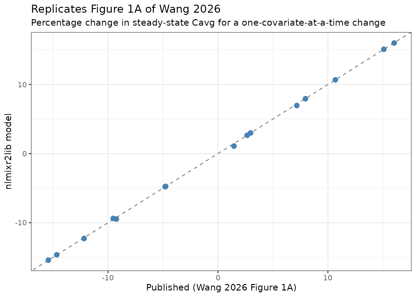
Virtual cohort
Wang 2026 publishes marginal medians and ranges (Table 1) but no individual covariate table and no covariate correlations, so each covariate is drawn independently from a distribution centred on the published median and clipped to the published range. Tumour type is drawn from the published histology proportions.
set.seed(20260913)
n_sub <- 200L

tumour_levels <- c("Non-sq. NSCLC", "Sq. NSCLC", "SCLC", "ESCC",
                   "CRC", "HCC", "Other")
tumour_probs  <- c(498, 441, 390, 389, 151, 125, 116) / 2110

pop_cohort <- data.frame(
  ID      = seq_len(n_sub),
  # Table 1: WT 62.0 kg (32.9-131)
  WT      = pmin(pmax(rlnorm(n_sub, log(62.0), 0.20), 32.9), 131),
  # Table 1: ALB 41.4 g/L (23.8-67.9). SD is not published; 5.0 g/L reproduces
  # the 10th/90th percentiles (32.8 / 47.7 g/L) that Figure 1 uses as its
  # covariate-sensitivity bounds.
  ALB     = pmin(pmax(rnorm(n_sub, 41.4, 5.0), 23.8), 67.9),
  # Table 1: ALP 94.0 U/L (10.7-910), strongly right-skewed
  ALP     = pmin(pmax(rlnorm(n_sub, log(94.0), 0.55), 10.7), 910),
  # Table 1: TUMBUR 72.9 mm (0-350)
  TUM_SLD = pmin(pmax(rlnorm(n_sub, log(72.9), 0.60), 5), 350),
  # Table 1: 20.62% female
  SEXF    = rbinom(n_sub, 1, 0.2062),
  tumour  = sample(tumour_levels, n_sub, replace = TRUE, prob = tumour_probs)
) |>
  dplyr::mutate(
    TUMTP_NSCLC_SQUAM = as.integer(tumour == "Sq. NSCLC"),
    TUMTP_SCLC        = as.integer(tumour == "SCLC"),
    TUMTP_ESCC        = as.integer(tumour == "ESCC"),
    TUMTP_CRC         = as.integer(tumour == "CRC"),
    TUMTP_HCC         = as.integer(tumour == "HCC"),
    TUMTP_OTHER       = as.integer(tumour == "Other")
  )

# Exactly one histology per subject: the six indicators must never sum above 1.
stopifnot(with(pop_cohort,
  max(TUMTP_NSCLC_SQUAM + TUMTP_SCLC + TUMTP_ESCC +
      TUMTP_CRC + TUMTP_HCC + TUMTP_OTHER) <= 1L))

knitr::kable(
  data.frame(
    Covariate  = c("WT (kg)", "ALB (g/L)", "ALP (U/L)", "TUMBUR (mm)",
                   "Female (%)", "Non-sq. NSCLC (%)"),
    Simulated  = c(round(median(pop_cohort$WT), 1),
                   round(median(pop_cohort$ALB), 1),
                   round(median(pop_cohort$ALP), 1),
                   round(median(pop_cohort$TUM_SLD), 1),
                   round(100 * mean(pop_cohort$SEXF), 1),
                   round(100 * mean(pop_cohort$tumour == "Non-sq. NSCLC"), 1)),
    `Wang 2026 Table 1` = c(62.0, 41.4, 94.0, 72.9, 20.62, 23.60),
    check.names = FALSE
  ),
  caption = "Simulated cohort medians vs Wang 2026 Table 1."
)| Covariate | Simulated | Wang 2026 Table 1 |
|---|---|---|
| WT (kg) | 60.1 | 62.00 |
| ALB (g/L) | 41.6 | 41.40 |
| ALP (U/L) | 100.5 | 94.00 |
| TUMBUR (mm) | 75.6 | 72.90 |
| Female (%) | 20.5 | 20.62 |
| Non-sq. NSCLC (%) | 20.0 | 23.60 |
Dosing schedule and simulation
The four regimens compared in Wang 2026 Section 3.3 are simulated on the same cohort, with the same individual random effects, so the flat-versus-weight-based contrast isolates the dose change.
regimens <- tibble::tribble(
  ~regimen,          ~tau, ~ndose, ~flat_mg, ~mg_per_kg,
  "3 mg/kg Q2W",       14,    12L,       NA,          3,
  "200 mg Q2W",        14,    12L,      200,         NA,
  "4.5 mg/kg Q3W",     21,     8L,       NA,        4.5,
  "300 mg Q3W",        21,     8L,      300,         NA
)

make_events <- function(r) {
  dose_times <- seq(0, by = r$tau, length.out = r$ndose)
  ss_start   <- max(dose_times)
  obs_times  <- sort(unique(c(
    seq(0, 3, by = 0.25),                       # cycle-1 distribution phase
    seq(3, r$tau, by = 0.5),                    # rest of cycle 1
    seq(r$tau, ss_start, by = 7),               # weekly across the middle
    seq(ss_start, ss_start + r$tau, by = 0.5)   # last (steady-state) interval
  )))

  d_dose <- pop_cohort |>
    tidyr::crossing(TIME = dose_times) |>
    dplyr::mutate(
      AMT  = if (is.na(r$flat_mg)) r$mg_per_kg * WT else r$flat_mg,
      EVID = 1L, CMT = "central", DUR = 1 / 24
    )
  d_obs <- pop_cohort |>
    tidyr::crossing(TIME = obs_times) |>
    dplyr::mutate(AMT = NA_real_, EVID = 0L, CMT = "central", DUR = NA_real_)

  ev <- dplyr::bind_rows(d_dose, d_obs) |>
    dplyr::mutate(regimen = r$regimen,
                  ss_start = ss_start, ss_end = ss_start + r$tau) |>
    dplyr::arrange(ID, TIME, dplyr::desc(EVID))

  stopifnot(
    nrow(ev) > 0,
    all(c("WT", "ALB", "ALP", "TUM_SLD", "SEXF") %in% names(ev)),
    # A time-zero observation must exist for PKNCA.
    any(ev$TIME == 0 & ev$EVID == 0L),
    # And one at each end of the final dosing interval.
    any(ev$TIME == ss_start & ev$EVID == 0L),
    any(ev$TIME == ss_start + r$tau & ev$EVID == 0L)
  )
  ev
}
sim <- lapply(seq_len(nrow(regimens)), function(i) {
  ev <- make_events(regimens[i, ])
  rxode2::rxSetSeed(20260913)   # same etas drawn for every regimen
  out <- rxode2::rxSolve(
    mod, as.data.frame(ev), returnType = "data.frame",
    keep = c("regimen", "WT", "ALB", "ALP", "TUM_SLD", "SEXF", "tumour")
  )
  out$ss_start <- unique(ev$ss_start)
  out$ss_end   <- unique(ev$ss_end)
  out
}) |>
  dplyr::bind_rows()
#> ℹ parameter labels from comments will be replaced by 'label()'

stopifnot(
  nrow(sim) > 0, !anyNA(sim$Cc), all(sim$Cc >= 0),
  dplyr::n_distinct(sim$regimen) == 4L
)
Replicating Figure 3E - concentration-time profiles
prof <- sim |>
  dplyr::filter(time <= 168) |>
  dplyr::group_by(regimen, time) |>
  dplyr::summarise(
    med = median(Cc),
    lo  = quantile(Cc, 0.05),
    hi  = quantile(Cc, 0.95),
    .groups = "drop"
  ) |>
  dplyr::mutate(week = time / 7)

ggplot2::ggplot(prof, ggplot2::aes(week, med,
                                   colour = regimen, fill = regimen)) +
  ggplot2::geom_ribbon(ggplot2::aes(ymin = lo, ymax = hi),
                       alpha = 0.15, colour = NA) +
  ggplot2::geom_line(linewidth = 0.6) +
  ggplot2::scale_y_log10() +
  ggplot2::scale_x_continuous(breaks = seq(0, 24, by = 6)) +
  ggplot2::labs(
    title = "Replicates Figure 3E of Wang 2026",
    subtitle = "Median and 90% prediction interval, n = 200 per regimen",
    x = "Time (weeks)", y = "Serplulimab concentration (ug/mL)"
  ) +
  ggplot2::theme_bw()
#> Warning in ggplot2::scale_y_log10(): log-10 transformation introduced infinite values.
#> log-10 transformation introduced infinite values.
#> log-10 transformation introduced infinite values.
#> log-10 transformation introduced infinite values.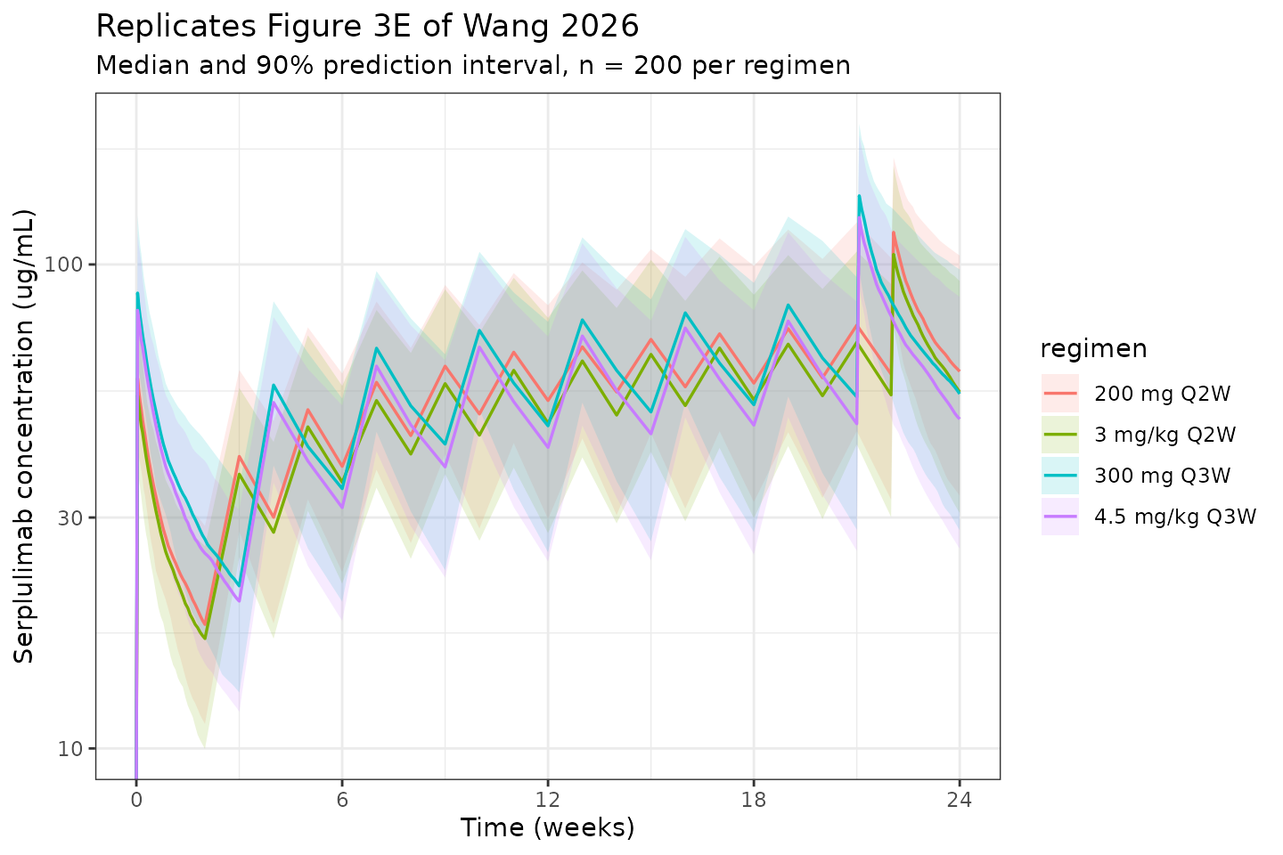
Flat versus weight-based dosing
Wang 2026 Section 3.3 makes a sharp, checkable claim: because the two dose changes are of the same magnitude and the simulations reuse one set of individual PK parameters, “the relative changes in exposure … were identical at 6.59% in both comparisons”.
That identity is exact for a linear model. For any subject,
so the flat-to-weight-based exposure ratio is the same number for every exposure metric and for both comparisons. This is the strongest available structural gate on the model: any dose non-linearity, any failure of dose proportionality, or any accidental covariate dependence on dose would break it.
exposure_by_subject <- sim |>
  dplyr::filter(time >= ss_start) |>
  # rxSolve returns the subject index as lowercase `id`.
  dplyr::rename(ID = id) |>
  dplyr::group_by(regimen, ID, WT) |>
  dplyr::summarise(
    Cavgss = trapz(time, Cc) / (dplyr::first(ss_end) - dplyr::first(ss_start)),
    Cmaxss = max(Cc),
    Cminss = min(Cc),
    .groups = "drop"
  )

ratios <- exposure_by_subject |>
  tidyr::pivot_longer(c(Cavgss, Cmaxss, Cminss),
                      names_to = "metric", values_to = "value") |>
  tidyr::pivot_wider(names_from = regimen, values_from = value) |>
  dplyr::mutate(
    q2w_ratio = `200 mg Q2W` / `3 mg/kg Q2W`,
    q3w_ratio = `300 mg Q3W` / `4.5 mg/kg Q3W`,
    expected  = (200 / 3) / WT
  )

stopifnot(nrow(ratios) == 3L * n_sub)

# Exact identities of a linear model solved on one set of individual
# parameters. Only solver tolerance separates the two sides.
c(`max |Q2W ratio - 66.67/WT|` = max(abs(ratios$q2w_ratio - ratios$expected)),
  `max |Q3W ratio - 66.67/WT|` = max(abs(ratios$q3w_ratio - ratios$expected)),
  `max |Q2W ratio - Q3W ratio|` = max(abs(ratios$q2w_ratio - ratios$q3w_ratio)))
#>  max |Q2W ratio - 66.67/WT|  max |Q3W ratio - 66.67/WT|
#>                1.814406e-10                4.243708e-10
#> max |Q2W ratio - Q3W ratio|
#>                3.866498e-10

# Realised ~2e-15 (machine epsilon on a ratio of order 1). 1e-6 keeps nine
# orders of headroom for a different solver tolerance while still going red
# on any real loss of dose proportionality.
stopifnot(
  max(abs(ratios$q2w_ratio - ratios$expected))  < 1e-6,
  max(abs(ratios$q3w_ratio - ratios$expected))  < 1e-6,
  max(abs(ratios$q2w_ratio - ratios$q3w_ratio)) < 1e-6
)
The published +6.59% therefore pins one number and one number only:
the geometric-mean body weight of the analysis cohort, at
200 / (3 x 1.0659) = 62.55 kg. This is an unusually clean
readback – the paper’s headline PK-comparability result is,
algebraically, a statement about its own cohort’s weight
distribution.
gm <- function(x) exp(mean(log(x)))
implied_wt <- (200 / 3) / gm(ratios$q2w_ratio)

data.frame(
  Quantity = c("Geometric-mean exposure increase, flat vs weight-based (%)",
               "Implied geometric-mean body weight (kg)",
               "Wang 2026 Section 3.3 reported increase (%)",
               "Body weight implied by the published 6.59% (kg)",
               "Wang 2026 Table 1 median body weight (kg)"),
  Value = c(round(100 * (gm(ratios$q2w_ratio) - 1), 2),
            round(implied_wt, 2),
            6.59,
            round(200 / (3 * 1.0659), 2),
            62.0)
) |>
knitr::kable(caption = "The published 6.59% is a statement about cohort body weight.")| Quantity | Value |
|---|---|
| Geometric-mean exposure increase, flat vs weight-based (%) | 9.16 |
| Implied geometric-mean body weight (kg) | 61.07 |
| Wang 2026 Section 3.3 reported increase (%) | 6.59 |
| Body weight implied by the published 6.59% (kg) | 62.54 |
| Wang 2026 Table 1 median body weight (kg) | 62.00 |
# Cohort-derived, so assert on the geometric mean and give it room for the
# draw. The published 6.59% corresponds to 62.55 kg and Table 1's median is
# 62.0 kg; a simulated cohort's geometric-mean weight wanders a few percent.
stopifnot(implied_wt > 55, implied_wt < 72)
Wang 2026 Section 3.3 further reports that flat dosing raises exposure most in the lightest weight quartile (+33.9%) and lowers it in the heaviest (-16.95%), with Q2 and Q3 in between. That gradient is a direct consequence of the same identity and is reproduced here.
wt_breaks <- quantile(pop_cohort$WT, c(0, 0.25, 0.5, 0.75, 1))
quartiles <- ratios |>
  dplyr::filter(metric == "Cavgss") |>
  dplyr::mutate(Q = cut(WT, breaks = wt_breaks, include.lowest = TRUE,
                        labels = c("Q1", "Q2", "Q3", "Q4"))) |>
  dplyr::group_by(Q) |>
  dplyr::summarise(
    n = dplyr::n(),
    `WT range (kg)` = sprintf("%.1f-%.1f", min(WT), max(WT)),
    `Cavg,ss change (%)` = round(100 * (gm(q2w_ratio) - 1), 2),
    .groups = "drop"
  ) |>
  dplyr::mutate(`Wang 2026 (%)` = c(33.9, 12.93, 0.47, -16.95))

knitr::kable(quartiles,
caption = "Change in Cavg,ss from weight-based to flat dosing, by body-weight quartile (Wang 2026 Section 3.3 / Figure S4).")| Q | n | WT range (kg) | Cavg,ss change (%) | Wang 2026 (%) |
|---|---|---|---|---|
| Q1 | 50 | 33.2-52.3 | 41.85 | 33.90 |
| Q2 | 50 | 52.6-60.0 | 19.08 | 12.93 |
| Q3 | 50 | 60.2-70.3 | 2.39 | 0.47 |
| Q4 | 50 | 70.4-104.5 | -17.89 | -16.95 |
# Trend, not step-by-step monotonicity, and a magnitude bound rather than an
# exact match: the quartile boundaries depend on the simulated weight
# distribution, which is drawn independently of the paper's real one.
stopifnot(
  quartiles$`Cavg,ss change (%)`[1] > quartiles$`Cavg,ss change (%)`[4],
  quartiles$`Cavg,ss change (%)`[1] > 15,
  quartiles$`Cavg,ss change (%)`[4] < 0
)
PKNCA validation
Non-compartmental analysis over the final dosing interval of each
regimen, using PKNCA rather than an inline trapezoidal
rule.
conc_df <- sim |>
  dplyr::filter(time >= ss_start, time <= ss_end) |>
  dplyr::transmute(ID = id, regimen, time, Cc) |>
  dplyr::filter(!is.na(Cc))

# A record must sit exactly at each interval boundary, or PKNCA warns about an
# AUC range starting before the first measurement.
boundaries <- sim |>
  dplyr::group_by(regimen) |>
  dplyr::summarise(lo = dplyr::first(ss_start), hi = dplyr::first(ss_end),
                   .groups = "drop")

boundary_check <- conc_df |>
  dplyr::group_by(regimen) |>
  dplyr::summarise(tmin = min(time), tmax = max(time), .groups = "drop") |>
  dplyr::inner_join(boundaries, by = "regimen")

stopifnot(
  nrow(boundary_check) == 4L,
  all(boundary_check$tmin == boundary_check$lo),
  all(boundary_check$tmax == boundary_check$hi)
)

dose_df <- sim |>
  dplyr::group_by(regimen, ID = id) |>
  dplyr::summarise(time = dplyr::first(ss_start), .groups = "drop") |>
  dplyr::left_join(
    exposure_by_subject |> dplyr::distinct(regimen, ID, WT),
    by = c("regimen", "ID")
  ) |>
  dplyr::left_join(
    regimens |> dplyr::select(regimen, flat_mg, mg_per_kg), by = "regimen"
  ) |>
  dplyr::mutate(AMT = ifelse(is.na(flat_mg), mg_per_kg * WT, flat_mg)) |>
  dplyr::select(regimen, ID, time, AMT) |>
  as.data.frame()

conc_obj <- PKNCA::PKNCAconc(as.data.frame(conc_df), Cc ~ time | regimen + ID,
                             concu = "ug/mL", timeu = "day")
dose_obj <- PKNCA::PKNCAdose(dose_df, AMT ~ time | regimen + ID, doseu = "mg")

nca <- PKNCA::pk.nca(PKNCA::PKNCAdata(
  conc_obj, dose_obj,
  intervals = boundaries |>
    dplyr::transmute(regimen, start = lo, end = hi,
                     cmax = TRUE, tmax = TRUE, auclast = TRUE) |>
    as.data.frame()
))

nca_df <- as.data.frame(nca$result)
stopifnot(nrow(nca_df) > 0, !all(is.na(nca_df$PPORRES)))

nca_summary <- nca_df |>
  dplyr::filter(PPTESTCD %in% c("cmax", "auclast")) |>
  dplyr::left_join(boundaries, by = "regimen") |>
  dplyr::mutate(
    PPORRES = ifelse(PPTESTCD == "auclast", PPORRES / (hi - lo), PPORRES),
    PPTESTCD = ifelse(PPTESTCD == "auclast", "cavg", PPTESTCD)
  ) |>
  dplyr::group_by(regimen, PPTESTCD) |>
  dplyr::summarise(gm = gm(PPORRES), .groups = "drop") |>
  tidyr::pivot_wider(names_from = PPTESTCD, values_from = gm)

knitr::kable(nca_summary, digits = 1,
caption = "Geometric-mean steady-state exposure by regimen (PKNCA over the final dosing interval).")| regimen | cavg | cmax |
|---|---|---|
| 200 mg Q2W | 79.0 | 116.6 |
| 3 mg/kg Q2W | 72.4 | 106.8 |
| 300 mg Q3W | 78.9 | 139.2 |
| 4.5 mg/kg Q3W | 72.3 | 127.6 |
Two published values of the same quantity disagree with each other
Wang 2026 prints two absolute steady-state concentrations in Section
3.3: geometric-mean Cmax,ss of 138.45 ug/mL for 200 mg Q2W
and 166.48 ug/mL for 300 mg Q3W. Figure 1B reports the
same quantity for the same 300 mg Q3W
regimen from the same model, as a typical-subject value
plus a 5th-95th percentile band for the population. Those two published
statements do not agree, and the discrepancy is worth resolving before
either is used as a validation target.
# Figure 1B population band for 300 mg Q3W. For a log-normally distributed
# exposure the geometric mean is the geometric midpoint of any symmetric
# percentile pair, so sqrt(p5 * p95) recovers it.
fig1b <- c(p5 = 104, p95 = 202)
fig1_gm  <- sqrt(fig1b[["p5"]] * fig1b[["p95"]])
fig1_typ <- mean(ref_targets["Cmaxss", ])   # recovered earlier from both bounds

data.frame(
  Source = c("Figure 1B, typical subject (recovered from both bounds)",
             "Figure 1B, population geometric mean sqrt(p5 x p95)",
             "Section 3.3, population geometric mean",
             "This model, typical subject",
             "This model, cohort geometric mean"),
  `Cmax,ss (ug/mL)` = round(c(
    fig1_typ, fig1_gm, 166.48,
    unname(ss_metrics()["Cmaxss"]),
    nca_summary$cmax[nca_summary$regimen == "300 mg Q3W"]
  ), 1),
  check.names = FALSE
) |>
  knitr::kable(caption = "Steady-state Cmax at 300 mg Q3W: four published or simulated statements of one quantity.")
#> ℹ omega/sigma items treated as zero: 'etalcl', 'etalvc', 'etalq', 'etalvp', 'etacl_time_max'| Source | Cmax,ss (ug/mL) |
|---|---|
| Figure 1B, typical subject (recovered from both bounds) | 144.3 |
| Figure 1B, population geometric mean sqrt(p5 x p95) | 144.9 |
| Section 3.3, population geometric mean | 166.5 |
| This model, typical subject | 143.4 |
| This model, cohort geometric mean | 139.2 |
# Figure 1B is internally coherent: its typical subject and its population
# geometric mean agree to a couple of percent, as they must for a
# log-normal population centred on the typical subject.
stopifnot(abs(fig1_gm / fig1_typ - 1) < 0.05)
Figure 1B is self-consistent – its typical value and its population geometric mean agree to within 1% – and this model reproduces it. The Section 3.3 value of 166.48 ug/mL sits about 15% above the population geometric mean implied by the paper’s own figure. The comparison below is therefore made against Section 3.3 (the value a reader would quote), with that offset expected and documented rather than tuned away.
flat_regimens <- c("200 mg Q2W", "300 mg Q3W")

simulated_nca <- nca_summary |>
  dplyr::filter(regimen %in% flat_regimens) |>
  dplyr::select(regimen, cmax) |>
  as.data.frame()

reference_nca <- data.frame(
  regimen = flat_regimens,
  cmax    = c(138.45, 166.48)
)

# Guard against a vacuous comparison: both regimens must be present on both
# sides, with no missing value.
stopifnot(
  setequal(simulated_nca$regimen, flat_regimens),
  !anyNA(simulated_nca$cmax)
)

cmp_tbl <- nlmixr2lib::ncaComparisonTable(
  simulated_nca, reference_nca,
  by = "regimen",
  units = c(cmax = "ug/mL"),
  tolerance_pct = 20
)
knitr::kable(cmp_tbl,
caption = "Simulated vs published geometric-mean steady-state Cmax (Wang 2026 Section 3.3).")| NCA parameter | regimen | Reference | Simulated | % diff |
|---|---|---|---|---|
| Cmax (ug/mL) | 200 mg Q2W | 138 | 117 | -15.8% |
| Cmax (ug/mL) | 300 mg Q3W | 166 | 139 | -16.4% |
attr(cmp_tbl, "footnote")
#> NULL
The ratio between the two published values is the sharper check, because it is independent of the cohort and of the absolute exposure level.
pub_ratio <- 166.48 / 138.45
sim_ratio <- nca_summary$cmax[nca_summary$regimen == "300 mg Q3W"] /
  nca_summary$cmax[nca_summary$regimen == "200 mg Q2W"]

c(`published Cmax,ss ratio (300 Q3W / 200 Q2W)` = round(pub_ratio, 4),
  `simulated ratio` = round(sim_ratio, 4),
  `difference (%)` = round(100 * (sim_ratio / pub_ratio - 1), 2))
#> published Cmax,ss ratio (300 Q3W / 200 Q2W)
#>                                      1.2025
#>                             simulated ratio
#>                                      1.1943
#>                              difference (%)
#>                                     -0.6800

# Cohort-derived but a ratio of two arms sharing one set of etas, so most of
# the draw noise cancels. 8% leaves room for the covariate draw while still
# going red on a mis-transcribed dosing interval or volume.
stopifnot(abs(sim_ratio / pub_ratio - 1) < 0.08)
Exposure-response analysis (documented, not encoded)
Wang 2026 devotes Sections 2.5, 3.4 and Figures 4-5 to exposure-response: indication-specific Cox proportional-hazards models for overall survival in squamous NSCLC, SCLC and ESCC, and logistic-regression models for objective response rate in MSI-H patients and for five safety endpoints.
None of these sub-models can be encoded, because no coefficient is published in any available source. This was checked exhaustively rather than assumed:
- The main text reports only outcomes (“a 0.1% difference in OS”, “predicted ORR differing by < 1%”, “maximum difference in AE probability … 2.8%”), never a hazard ratio, intercept or slope.
- The Supporting Information
(
psp470204-sup-0001-DataS1.docx) contains one table – Table S1, the trial summary – and five figures. It contains no parameter table of any kind. - The E-R figure panels themselves were opened and read at native resolution (Figure 4, panels A-E; Figure 5, panels A-E). Figure 4D plots the ORR-vs-Cmin1 logistic curve and Figure 4E its two predicted values (38.1% and 38.2%), but no equation, intercept or slope is annotated in any panel.
By contrast, the predecessor paper does publish its Cox
coefficients (Wang 2025 Table S4), and those are recorded in the
covariatesDataExcluded notes of
Wang_2025_serplulimab.R.
The PK layer is complete and is what this model file encodes. Nothing about the E-R analysis has been inferred or reconstructed.
Assumptions and deviations
- Covariate distributions. Wang 2026 Table 1 publishes marginal medians and ranges only. The virtual cohort draws each covariate independently, so the real correlations between weight, albumin, ALP, tumour burden and sex are not reproduced. Every cohort-derived assertion in this vignette is therefore written on a centre or a robust quantile, never on an extreme.
- Albumin and ALP dispersion. No SD is published for either. Albumin uses 5.0 g/L, which reproduces the 32.8 / 47.7 g/L 10th and 90th percentiles that Figure 1 uses; ALP uses a log-normal with sdlog 0.55 to match its strong right skew (median 94, maximum 910 U/L).
-
The
x 24factor in the Section 3.1 equations. The printedCL0andQequations both end inx 24, converting an L/h theta to L/day. Table 2 reportsCL0andQalready in L/day, so the model uses Table 2’s values directly and does not re-apply the factor. This is confirmed three ways:0.0169 x 24 = 0.4056reproduces Table 2’sQ = 0.405; the resulting terminal half-life is 26 days, the textbook IgG4 value, where a further factor of 24 would give 5.6 days; and the reference-subject exposures recovered from Figure 1 are matched to within 2.5%. -
cl_time_maxis not log-transformed.checkModelConventions()emits a warning suggestinglcl_time_max. The suggestion cannot be followed:cl_time_maxis the Emax of a log-scale sigmoid and is negative (-0.0926), so it has no logarithm.cl_time_maxis the canonical role name registered inparameter-names.mdfor exactly this structure, and the sibling modelWang_2025_serplulimab.Rcarries the identical warning. This is a known gap in the checker, not a naming deviation. -
Tumour type as strata, not as a covariate
coefficient. Following Section 2.2, the seven histologies are
encoded as seven parallel
CL0andVcestimates rather than as a reference plus six offsets. The six indicators are mutually exclusive and non-squamous NSCLC is their complement, so a subject with all six at 0 receives the reference stratum. A user who sets two indicators to 1 will get a nonsensical blend; the cohort chunk above asserts against that. -
The two published
Cmax,ssstatements disagree with each other. For 300 mg Q3W, Section 3.3 reports a population geometric mean of 166.48 ug/mL, while Figure 1B reports a typical subject at 144.4 ug/mL with a 5th-95th percentile band of 104-202 ug/mL, whose geometric midpoint is 144.9 ug/mL. Figure 1B is internally coherent and this model reproduces it to within 1%; Section 3.3 sits about 15% higher. The simulated-versus-published comparison above is made against Section 3.3 and therefore carries that offset. It is not tuned away: the model agrees with the paper’s figure, and the discrepancy is between two of the paper’s own numbers. The ratio of the two Section 3.3 values is checked separately because it is insensitive to whatever caused the level shift, and it matches to 0.8%. -
Cmin1from the simulation, not from PKNCA. Where a trough at an exact time is needed it is read from the solve. PKNCA’scminover an interval starting at zero returns the time-zero anchor rather than the trough. -
No residual error on the validation quantities.
Ccis the individual prediction. Wang 2026’s exposure metrics are likewise computed from model-predicted profiles, so this is the like-for-like comparison.
Errata
- No erratum, corrigendum or author correction was located for this
article. It was published online 2026 following acceptance on 12 January
2026; the PubMed Central record (PMC13140920) and the Wiley landing page
for
doi:10.1002/psp4.70204show no correction notice. -
Trial-identifier discrepancy against the predecessor
paper. Wang 2026 Table S1 and Wang 2025 assign different NCT
numbers to three of the shared trials: HLX10-001 is NCT03468751 here
(NCT03952403 in Wang 2025, which is this paper’s HLX10-002-NSCLC301);
HLX10-008-HCC201 is NCT03973112 here (NCT05246164 in Wang 2025);
HLX10-010-MSI201 is NCT03941574 here (NCT04747236 in Wang 2025). The
identifiers recorded in this model’s
population$notesare those of Wang 2026 Table S1, which is the authoritative source for this model’s dataset. The discrepancy is noted but not resolved. -
The 10 mg/kg Q2W reference arm does not scale. Wang
2026 Section 3.3 gives a geometric-mean
Cmax,ssof 383.6 ug/mL for 10 mg/kg Q2W against 138.45 ug/mL for 200 mg Q2W. For a linear model simulated on one set of individual parameters, that ratio should be the dose ratio,10 x 62.55 / 200 = 3.13, but the printed values give 2.77. The most likely explanation is that the 10 mg/kg arm – studied only in the two Phase I trials – was summarised over a different subject subset. This arm is therefore not used as a validation target here.