Voriconazole (Suetsugu 2021)

Model and source

• Citation: Suetsugu K, Muraki S, Fukumoto J, Matsukane R, Mori Y, Hirota T, Miyamoto T, Egashira N, Akashi K, Ieiri I. Effects of Letermovir and/or Methylprednisolone Coadministration on Voriconazole Pharmacokinetics in Hematopoietic Stem Cell Transplantation: A Population Pharmacokinetic Study. Drugs R D. 2021;21(4):419-429. doi:10.1007/s40268-021-00365-0
• Description: Steady-state Michaelis-Menten population PK model relating the voriconazole steady-state trough concentration to the daily maintenance dose in Japanese adult allogeneic haematopoietic stem cell transplant recipients (Suetsugu 2021; n = 47, 216 trough samples). The model is algebraic – Css_trough = Km * F * dose / (Vmax - F * dose), with the daily dose supplied as the DOSE_VORI_MGD covariate and F fixed to 1 – because every observation was a steady-state trough and no volume or absorption parameter was estimated. Vmax is 1.72-fold higher with concomitant letermovir and 1.30-fold higher with concomitant methylprednisolone (multiplicative), with log-normal IIV on Vmax and an additive residual error. No steady state exists when F * dose >= Vmax; the equation then returns a negative or infinite value.
• Article: https://doi.org/10.1007/s40268-021-00365-0 (open access, PMC8602551)

Suetsugu et al. analysed routine voriconazole therapeutic-drug-monitoring troughs from adult allogeneic haematopoietic stem cell transplant (allo-HSCT) recipients to quantify the drug-drug interaction with letermovir, a cytomegalovirus prophylactic that induces CYP2C19 and CYP2C9. Because every observation was a steady-state trough, the authors did not fit a compartmental model. They fitted the steady-state Michaelis-Menten relation between the daily maintenance dose and the trough concentration directly (Eq. 1):

$$C_{ss,\,trough} = \frac{K_m \times F \times \text{Daily dose}}{V_{max} - F \times \text{Daily dose}}$$

with $F$ fixed to 1 and $V_{max,i} = 670 \times 1.72^{LMV_i} \times 1.30^{mPSL_i}$ (Eq. 4), where LMV and mPSL flag concomitant letermovir and methylprednisolone.

The packaged model is therefore algebraic: it has no time dimension, no compartments and no dosing events. The daily dose enters as the covariate DOSE_VORI_MGD (mg/day), and each observation row returns the steady-state trough Cc (mg/L) for that dose level and co-medication state.

Population

The model was fitted to 216 steady-state voriconazole troughs from 47 Japanese adults (23 male, 24 female; median age 51 years, range 22-69; median weight 55.0 kg, range 31.3-90.3) who underwent allo-HSCT at Kyushu University Hospital between April 2016 and March 2020 with tacrolimus graft-versus-host disease prophylaxis (Suetsugu 2021 Section 2.1 and Table 1). Voriconazole was given for treatment (n = 33) or prophylaxis (n = 14) of invasive fungal infection, orally (38), intravenously (1) or both (8). Nineteen patients received letermovir (71 of the 216 samples; Fig. 1), 18 methylprednisolone, 19 prednisolone and 2 dexamethasone. Patients starting voriconazole more than 100 days after HSCT, under 20 years old, or with liver dysfunction were excluded, as were concentrations within 5 days of starting voriconazole.

The same information is available programmatically:

str(rxode2::rxode(readModelDb("Suetsugu_2021_voriconazole"))$population)
#> ℹ parameter labels from comments will be replaced by 'label()'
#> List of 17
#>  $ species        : chr "human"
#>  $ n_subjects     : int 47
#>  $ n_studies      : int 1
#>  $ n_observations : int 216
#>  $ age_range      : chr "22-69 years"
#>  $ age_median     : chr "51 years"
#>  $ weight_range   : chr "31.3-90.3 kg"
#>  $ weight_median  : chr "55.0 kg"
#>  $ sex_female_pct : num 51.1
#>  $ race_ethnicity : chr "Japanese (single centre, Kyushu University Hospital, Fukuoka)"
#>  $ disease_state  : chr "Adult allogeneic haematopoietic stem cell transplant recipients (April 2016 - March 2020) on tacrolimus graft-v"| __truncated__
#>  $ dose_range     : chr "Voriconazole maintenance doses from routine care; 38 patients oral only, 1 intravenous only, 8 both (28 of 216 "| __truncated__
#>  $ co_medication  : chr "Letermovir 19 patients; methylprednisolone 18, prednisolone 19, dexamethasone 2; PPIs rabeprazole 16, esomepraz"| __truncated__
#>  $ regions        : chr "Japan (Kyushu University Hospital, Fukuoka)"
#>  $ sampling_window: chr "Steady-state trough concentrations only; concentrations within 5 days of voriconazole initiation were excluded (Section 2.2)."
#>  $ assay          : chr "UPLC or UPLC-MS/MS outsourced to SRL (LLOQ 0.1 mg/L) or LSI Medience (LLOQ 0.3 mg/L); CV < 15% (Section 2.2)."
#>  $ notes          : chr "Retrospective single-centre TDM analysis; NONMEM 7.4.3 FOCE-I. Evaluation by GOF, case-deletion diagnostics and"| __truncated__

Source trace

The per-parameter origin is recorded as an in-file comment next to each ini() entry in inst/modeldb/specificDrugs/Suetsugu_2021_voriconazole.R.

Equation / parameter	Value	Source location
Steady-state trough equation	$K_m F D / (V_{max} - F D)$	Eq. 1, Section 2.5
Categorical covariate form	$P = P_{pop} \times \theta^X$	Eq. 3, Section 2.6
Final $V_{max}$ equation	$670 \times 1.72^{LMV} \times 1.30^{mPSL}$	Eq. 4, Section 3.3
lkm	log(1.97) mg/L	Table 2, Km 1.97 ug/mL
lvmax	log(670) mg/day	Table 2, Vmax 670 mg/day
lfdepot	fixed(log(1))	Section 2.5, ‘the F-value was set to 1’
e_conmed_letermovir_vmax	1.72	Table 2, ‘Effect of LMV on Vmax’
e_conmed_methylprednisolone_vmax	1.30	Table 2, ‘Effect of mPSL on Vmax’
etalvmax	0.05421 = log(1 + 0.236^2)	Table 2, IIV Vmax 23.6 CV%; exponential model (Section 2.5)
addSd	0.77 mg/L	Table 2, ‘Additive error (ug/mL)’ 0.77

Typical-value check against the closed form

With the random effects zeroed, the model must return exactly Eq. 1 with the Table 2 typical values. The event table puts one observation row per dose level and co-medication state on a single subject; time is only a row index, since the model has no time dimension.

mod <- readModelDb("Suetsugu_2021_voriconazole")

grid <- tidyr::expand_grid(
  group = c("No DDI", "with LMV", "with mPSL"),
  dose = c(300, 400, 500, 600)
) |>
  mutate(
    CONMED_LETERMOVIR = as.integer(group == "with LMV"),
    CONMED_METHYLPREDNISOLONE = as.integer(group == "with mPSL")
  )

ev_typ <- grid |>
  transmute(
    id = 1L,
    time = seq_len(n()),
    evid = 0L,
    amt = 0,
    DOSE_VORI_MGD = dose,
    CONMED_LETERMOVIR,
    CONMED_METHYLPREDNISOLONE
  )

typ <- as.data.frame(rxode2::rxSolve(
  rxode2::zeroRe(mod),
  events = ev_typ,
  returnType = "data.frame"
))
#> ℹ parameter labels from comments will be replaced by 'label()'
#> ℹ omega/sigma items treated as zero: 'etalvmax'
stopifnot(nrow(typ) == nrow(grid))

vmax_typ <- 670 * 1.72^grid$CONMED_LETERMOVIR * 1.30^grid$CONMED_METHYLPREDNISOLONE
grid$closed_form <- 1.97 * grid$dose / (vmax_typ - grid$dose)
grid$model <- typ$Cc

# Same parameters on both sides, so the only difference is floating point.
stopifnot(all(abs(grid$model - grid$closed_form) < 1e-8))

grid |>
  select(group, dose, model) |>
  tidyr::pivot_wider(names_from = group, values_from = model) |>
  dplyr::rename("Daily dose (mg)" = dose) |>
  knitr::kable(digits = 2, caption = "Typical steady-state trough (mg/L).")

Typical steady-state trough (mg/L).

Daily dose (mg)	No DDI	with LMV	with mPSL
300	1.60	0.69	1.04
400	2.92	1.05	1.67
500	5.79	1.51	2.65
600	16.89	2.14	4.36

The typical values already show the paper’s conclusions: without an interacting co-medication 300-400 mg/day lands in the 1-5 mg/L target, while letermovir (Vmax x 1.72) pushes the typical trough at 300 mg/day below 1 mg/L. At 600 mg/day without letermovir or methylprednisolone the typical trough is 16.9 mg/L because the dose is about 10% below Vmax; the curve is steep there, and for patients whose individual Vmax is below 600 mg/day no steady state exists at all.

curve_grid <- tidyr::expand_grid(
  group = c("No DDI", "with LMV", "with mPSL"),
  dose = seq(100, 640, by = 10)
) |>
  mutate(
    CONMED_LETERMOVIR = as.integer(group == "with LMV"),
    CONMED_METHYLPREDNISOLONE = as.integer(group == "with mPSL")
  )
ev_curve <- curve_grid |>
  transmute(
    id = 1L,
    time = seq_len(n()),
    evid = 0L,
    amt = 0,
    DOSE_VORI_MGD = dose,
    CONMED_LETERMOVIR,
    CONMED_METHYLPREDNISOLONE
  )
curve_sim <- as.data.frame(rxode2::rxSolve(
  rxode2::zeroRe(mod),
  events = ev_curve,
  returnType = "data.frame"
))
#> ℹ parameter labels from comments will be replaced by 'label()'
#> ℹ omega/sigma items treated as zero: 'etalvmax'
stopifnot(nrow(curve_sim) == nrow(curve_grid))
curve_grid$Cc <- curve_sim$Cc

ggplot(curve_grid, aes(dose, Cc, colour = group)) +
  annotate("rect", xmin = -Inf, xmax = Inf, ymin = 1, ymax = 5, alpha = 0.15) +
  geom_line(linewidth = 0.8) +
  coord_cartesian(ylim = c(0, 15)) +
  labs(
    x = "Daily voriconazole dose (mg/day)",
    y = "Typical steady-state trough (mg/L)",
    colour = NULL
  ) +
  theme_bw()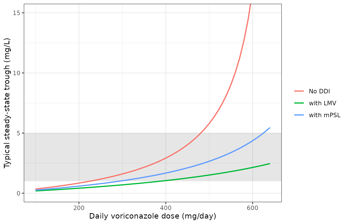

Typical steady-state trough versus daily dose (Eq. 1). The grey band is the 1-5 mg/L target. Each curve rises without bound as the dose approaches its Vmax (670, 871 and 1152 mg/day).

Virtual cohort and replication of Figure 4

Figure 4 of the paper shows Monte Carlo steady-state troughs (1000 per scenario) for 300-600 mg/day in three groups: no interacting co-medication, with letermovir, and with methylprednisolone. Each simulated patient needs only an individual Vmax (drawn from the IIV) and one trough with additive residual error. Here each scenario is simulated with 200 virtual patients.

Two properties of the equation shape the figure. When a patient’s Vmax is at or below the dose, Eq. 1 is negative or infinite: no steady state exists. With a 0.77 mg/L additive error, low troughs are also often simulated below zero. The paper does not say how it handled either case. Its box plots have no non-positive values and omit the no-DDI 500 and 600 mg/day scenarios. The no-DDI group has no steady state for about 10% of patients at 500 mg/day and about 32% at 600 mg/day. We reproduce the figure by keeping simulated troughs that have a steady state and are positive, and by showing only the scenarios the paper shows. Without that filter the medians do not match (see the Assumptions section).

n_per_arm <- 200L

scen <- tidyr::expand_grid(
  group = c("No DDI", "with LMV", "with mPSL"),
  dose = c(300, 400, 500, 600)
) |>
  filter(!(group == "No DDI" & dose > 400)) |>
  mutate(scenario = seq_len(n()))

ev_mc <- scen |>
  tidyr::uncount(n_per_arm) |>
  mutate(
    id = seq_len(n()),
    time = 0,
    evid = 0L,
    amt = 0,
    DOSE_VORI_MGD = dose,
    CONMED_LETERMOVIR = as.integer(group == "with LMV"),
    CONMED_METHYLPREDNISOLONE = as.integer(group == "with mPSL")
  )

rxode2::rxSetSeed(20211015)
mc <- as.data.frame(rxode2::rxSolve(mod, events = ev_mc, returnType = "data.frame"))
#> ℹ parameter labels from comments will be replaced by 'label()'
stopifnot(nrow(mc) == nrow(ev_mc))

mc <- ev_mc |>
  select(id, group, dose) |>
  left_join(mc |> select(id, vmax, sim), by = "id") |>
  mutate(retained = vmax > dose & sim > 0)

mc |>
  group_by(group, dose) |>
  summarise(
    `No steady state (%)` = 100 * mean(vmax <= dose),
    `Retained (%)` = 100 * mean(retained),
    .groups = "drop"
  ) |>
  dplyr::rename("Group" = group, "Daily dose (mg)" = dose) |>
  knitr::kable(digits = 1, caption = "Share of simulated troughs dropped before plotting.")

Share of simulated troughs dropped before plotting.

Group	Daily dose (mg)	No steady state (%)	Retained (%)
No DDI	300	0.0	95.0
No DDI	400	0.0	99.5
with LMV	300	0.0	85.0
with LMV	400	0.0	89.5
with LMV	500	0.0	96.0
with LMV	600	0.5	97.5
with mPSL	300	0.0	90.0
with mPSL	400	0.0	98.5
with mPSL	500	1.0	98.0
with mPSL	600	4.5	95.5

The published box-plot statistics come from the vector graphics of Figure 4 in the article PDF. They are the exact end points of each box (25th and 75th percentiles), its median line, and its whiskers (10th and 90th percentiles), converted to mg/L using the 1 and 5 mg/L target lines as the axis calibration.

fig4 <- read.table(header = TRUE, text = "
group      dose  q10    q25    q50    q75    q90
No_DDI     300   0.664  1.068  1.774  2.456  3.364
No_DDI     400   1.373  2.026  3.112  4.751  7.607
with_LMV   300   0.228  0.478  0.910  1.405  1.809
with_LMV   400   0.322  0.695  1.214  1.809  2.363
with_LMV   500   0.540  1.006  1.650  2.424  3.301
with_LMV   600   0.851  1.560  2.334  3.513  4.875
with_mPSL  300   0.353  0.664  1.183  1.746  2.276
with_mPSL  400   0.664  1.155  1.774  2.580  3.575
with_mPSL  500   1.125  1.871  2.764  3.949  6.369
with_mPSL  600   1.622  2.704  4.163  7.296  14.307
") |>
  mutate(group = sub("_", " ", group))

sim_q <- mc |>
  filter(retained) |>
  group_by(group, dose) |>
  summarise(
    q10 = quantile(sim, 0.10),
    q25 = quantile(sim, 0.25),
    q50 = quantile(sim, 0.50),
    q75 = quantile(sim, 0.75),
    q90 = quantile(sim, 0.90),
    .groups = "drop"
  )

ggplot(sim_q, aes(x = factor(dose))) +
  annotate("rect", xmin = -Inf, xmax = Inf, ymin = 1, ymax = 5, alpha = 0.15) +
  geom_boxplot(
    aes(ymin = q10, lower = q25, middle = q50, upper = q75, ymax = q90),
    stat = "identity",
    fill = "grey80",
    width = 0.6
  ) +
  geom_point(data = fig4, aes(y = q50), colour = "red", shape = 18, size = 3) +
  facet_grid(~group, scales = "free_x", space = "free_x") +
  coord_cartesian(ylim = c(0, 15)) +
  labs(x = "Daily dose (mg)", y = "Voriconazole concentration (mg/L)") +
  theme_bw()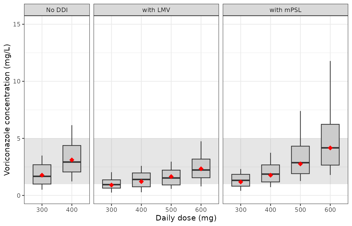

Replicates Figure 4 of Suetsugu 2021: simulated steady-state voriconazole troughs. Boxes are the 25th-75th percentiles with the median; whiskers are the 10th-90th percentiles. Red diamonds are the published medians. The grey band is the 1-5 mg/L target.

cmp <- sim_q |>
  tidyr::pivot_longer(q10:q90, names_to = "stat", values_to = "simulated") |>
  inner_join(
    fig4 |> tidyr::pivot_longer(q10:q90, names_to = "stat", values_to = "published"),
    by = c("group", "dose", "stat")
  ) |>
  mutate(pct_diff = 100 * (simulated - published) / published)
stopifnot(nrow(cmp) == 50L)

med_cmp <- cmp |> filter(stat == "q50")

med_cmp |>
  select(group, dose, published, simulated, pct_diff) |>
  dplyr::rename(
    "Group" = group,
    "Daily dose (mg)" = dose,
    "Published median (mg/L)" = published,
    "Simulated median (mg/L)" = simulated,
    "Difference (%)" = pct_diff
  ) |>
  knitr::kable(digits = 2, caption = "Median steady-state trough: simulation against Figure 4.")

Median steady-state trough: simulation against Figure 4.

Group	Daily dose (mg)	Published median (mg/L)	Simulated median (mg/L)	Difference (%)
No DDI	300	1.77	1.67	-5.59
No DDI	400	3.11	2.93	-5.92
with LMV	300	0.91	0.95	4.30
with LMV	400	1.21	1.40	15.35
with LMV	500	1.65	1.53	-7.26
with LMV	600	2.33	2.23	-4.45
with mPSL	300	1.18	1.32	11.75
with mPSL	400	1.77	1.87	5.41
with mPSL	500	2.76	2.87	3.84
with mPSL	600	4.16	4.17	0.19

# Bounds calibrated on 2000 independent 200-per-scenario cohorts drawn from
# the same model: |median of the ten median differences| reached at most
# 10.1% (99.9th percentile 7.1%), and the 80th percentile of the 50 absolute
# differences at most 19.2%. A Vmax of 607 instead of 670, a letermovir or
# methylprednisolone factor of 1.27 / 1.03, a residual SD of 0.077, or an IIV
# variance of 0.236 each failed the pair of bounds in every cohort tried.
stopifnot(
  # Structural: centre of the ten median differences.
  abs(median(med_cmp$pct_diff)) < 12,
  # Envelope over all 50 box-plot statistics, robust to the Monte Carlo noise
  # of 200 patients per scenario in the tails.
  quantile(abs(cmp$pct_diff), 0.8) < 25
)

With 200 000 patients per scenario the same filter reproduces all ten published medians within 3.2% and 49 of the 50 box-plot statistics within 10%; the exception is the with-methylprednisolone 600 mg/day 10th percentile (+13%) (checked while preparing this vignette). The remaining differences above come from Monte Carlo noise with 200 patients per scenario, which is largest at the 10th and 90th percentiles.

Target attainment

The paper’s dosing conclusion (Section 3.5) is that 300 or 400 mg/day reaches the 1-5 mg/L target without an interacting co-medication, 500 or 600 mg/day with letermovir, and 400 or 500 mg/day with methylprednisolone. The same retained simulations give:

pta <- mc |>
  filter(retained) |>
  group_by(group, dose) |>
  summarise(`In 1-5 mg/L (%)` = 100 * mean(sim >= 1 & sim <= 5), .groups = "drop") |>
  tidyr::pivot_wider(names_from = group, values_from = `In 1-5 mg/L (%)`) |>
  dplyr::rename("Daily dose (mg)" = dose)
options(knitr.kable.NA = "not shown")
knitr::kable(pta, digits = 0, caption = "Percentage of retained simulated troughs within 1-5 mg/L (no-DDI 500 and 600 mg/day are not shown in the paper).")

Percentage of retained simulated troughs within 1-5 mg/L (no-DDI 500 and 600 mg/day are not shown in the paper).

Daily dose (mg)	No DDI	with LMV	with mPSL
300	72	46	64
400	77	64	79
500	not shown	68	76
600	not shown	78	58

Why no PKNCA section

The model has no time dimension. It returns a single steady-state trough for each dose level, and there is no concentration-time profile to put through a non-compartmental analysis. The paper reports no NCA parameters. The model is validated against its closed form and against the paper’s own simulation (Figure 4).

Assumptions and deviations

• Algebraic encoding. The paper’s model is Eq. 1 itself; it estimates no volume of distribution or absorption rate, and none is invented here. The model therefore cannot produce concentration-time profiles, only steady-state troughs for a given daily dose.
• Daily dose as a covariate. Eq. 1 takes the daily maintenance dose as an input, so the packaged model reads it from the DOSE_VORI_MGD column (mg/day, summed over the day) on each observation row instead of from dosing events. Oral and intravenous doses are treated alike because the paper fixed F to 1 (Section 2.5). A sensitivity analysis with F = 0.459 (ESM-4) is not part of the final model and is not included.
• No steady state when dose >= Vmax. For patients whose individual Vmax is at or below the daily dose, Eq. 1 returns a negative or infinite value. The model returns that value unchanged, as the published equation does; users should treat such rows as “no steady state” (unbounded accumulation), not as concentrations.
• Handling of non-positive simulated troughs in Figure 4. The paper does not describe it. Keeping only troughs with a steady state and a positive value (after additive residual error) reproduces the published box plots. Keeping all values, or plotting the individual predictions without residual error, does not: for example, the with-letermovir 300 mg/day median is then 0.74 or 0.69 mg/L instead of the published 0.91 mg/L. The simulated values in this article use the filter that reproduces the paper.
• IIV scale. Table 2 reports the IIV of Vmax as 23.6 CV% for an exponential model. It is converted with omega^2 = log(1 + CV^2) = 0.05421; the alternative omega^2 = CV^2 = 0.0557 differs by 3% and cannot be told apart from Figure 4.
• Additive residual error. Table 2 gives the additive error in ug/mL (0.77), i.e. a standard deviation in concentration units, used as addSd.
• Screened covariates. Sex, age, body weight, albumin, CRP, PPIs, prednisolone and dexamethasone were screened and not retained. They are listed in covariatesDataExcluded for provenance and do not enter the model.
• Errata. No correction notice was found for this article in Europe PMC (checked 2026-09-29).