Estradiol whole-body PBPK and PBPK-LiverODE (Sier 2017)
Source:vignettes/articles/Sier_2017_estradiol.Rmd
Sier_2017_estradiol.RmdModel and source
- Citation: Sier JH, Thumser AE, Plant NJ. Linking physiologically-based pharmacokinetic and genome-scale metabolic networks to understand estradiol biology. BMC Syst Biol. 2017;11:141. doi:10.1186/s12918-017-0520-3. Executable model deposited by the authors as BioModels MODEL1711210001 (E2_PBPK_v7.3).
- Article: BMC Syst Biol 2017;11:141 (open access; Additional file 1 holds the reaction tables, balance equations and global quantities).
- Executable models deposited by the authors: BioModels MODEL1711210001 (PBPK) and MODEL1711210002 (PBPK-LiverODE).
Sier, Thumser and Plant built a whole-body physiologically-based pharmacokinetic model of 17-beta-estradiol (E2) in women and then replaced its single hepatic intrinsic-clearance term in two ways: with a mechanistic ODE network of hepatic estrogen metabolism (PBPK-LiverODE), and with a genome-scale metabolic network solved by flux-balance analysis (PBPK-GSMN). Two of the three are ODE systems and are packaged here:
| Model | Hepatic clearance | nlmixr2lib name |
|---|---|---|
| PBPK | first-order intrinsic clearance scaled to liver weight | Sier_2017_estradiol_pbpk |
| PBPK-LiverODE | 27 Michaelis-Menten conversions + 6 conjugate transporters, non-specific binding | Sier_2017_estradiol_liverode_pbpk |
| PBPK-GSMN | Recon2 flux-balance analysis coupled through a quasi-steady-state Petri net | not packaged (see below) |
Both packaged models share one skeleton: venous and arterial blood with explicit reversible E2 binding to SHBG and albumin; 16 tissues, well-mixed except the permeability-limited liver and the lumped uterus + ovaries compartment the paper calls “gonads”; estrogen-receptor binding in liver and gonad cells; zero-order E2 biosynthesis in the gonads; and first-order extra-hepatic clearance from the kidney. Organ volumes and blood flows follow the Bosgra 2012 anthropometric equations in body weight, height and age.
mod_pbpk <- readModelDb("Sier_2017_estradiol_pbpk")
mod_lode <- readModelDb("Sier_2017_estradiol_liverode_pbpk")
models <- list(PBPK = mod_pbpk, `PBPK-LiverODE` = mod_lode)
The observation Cc is free (unbound) venous E2
in nM, including the endogenous baseline. All states are
concentrations, and the deposited COPASI models give every compartment a
size of 1, so a dose in nmol entered into a dose compartment is
numerically its starting concentration. The paper enters the 0.3 mg i.v.
bolus as 1101 nmol into the i.v. dose compartment
(depot_iv) and the 2 mg and 4 mg oral doses as 7342 and
14685 nmol into the oral dose compartment (depot).
Population
There was no population fit. Both models are deterministic, with no
inter-individual variability and no residual error. The paper’s virtual
population is 1495 women aged 18-45 years whose weight and height come
from NHANES 2013-14 (Methods, “Virtual patient population”; Additional
file 1 Figure S7). Model output was compared with published clinical
means: Kuhnz 1993 (0.3 mg i.v. bolus in young women) and Lyrenas 1981 (2
mg and 4 mg oral, plasma followed for 50 h). Covariates are body weight
(WT, kg), height (HT, cm; the source equations
use metres and the model converts) and age (AGE, years).
The deposited models start every state at the endogenous steady state of
a 60 kg, 1.63 m, 35-year-old reference woman.
str(mod_pbpk()$population)
#> List of 9
#>  $ species       : chr "human"
#>  $ n_subjects    : int 1495
#>  $ n_studies     : int 2
#>  $ age_range     : chr "18-45 years (virtual population)"
#>  $ sex_female_pct: num 100
#>  $ disease_state : chr "healthy women (endogenous estradiol plus single exogenous doses)"
#>  $ dose_range    : chr "Single 0.3 mg i.v. bolus; single 2 mg or 4 mg oral dose"
#>  $ regions       : chr "United States (NHANES anthropometrics)"
#>  $ notes         : chr "Not a population fit: a deterministic mechanistic model with no inter-individual variability or residual error."| __truncated__
Source trace
Every ini() value carries an in-file comment naming its
source. The table collects them. “Suppl.” is Additional file 1;
“deposit” is the authors’ BioModels SBML for the variant in
question.
| Quantity | PBPK | PBPK-LiverODE | Source |
|---|---|---|---|
ksyn_gonads E2 biosynthesis (nM/h) |
2 | 2 | deposit ‘Gonads: E2 Biosynthesis’ k1 = 2 x 1 nM species; BioModels curator note |
kiv i.v. delivery (1/h) |
250 | 250 | main text Results; Suppl. v12 |
ka oral absorption (1/h) |
0.025 | 0.025 | main text Results; Suppl. v14 |
kfeces unabsorbed oral loss (1/h) |
0.01 | 0.01 | main text Results; Suppl. v37 |
clint_per_g intrinsic clearance (1/h per g liver) |
0.018466 | – | Suppl. v11 |
kcleh extra-hepatic clearance (1/h) |
5 | 5 | Suppl. v10 |
kperm_in_liver / kperm_out_liver
(1/h) |
1000 / 277.8 | 150 / 41.7 | main text Results; Suppl. v32 |
kperm_in_gonads / kperm_out_gonads
(1/h) |
1000 / 100 | 1000 / 100 | Suppl. v19; deposit |
kon_shbg / koff_shbg
|
3600 / 5400 | 3600 / 5400 | Suppl. v5, v48 |
kon_albumin / koff_albumin
|
3600 / 6.12e7 | 3600 / 6.12e7 | Suppl. v4, v47 |
kon_er_* / koff_er_* (liver and
gonads) |
3600 / 900 | 3600 / 900 | Suppl. v25 (liver); deposit (gonads) |
bl_shbg, bl_albumin total protein
(nM) |
40, 500000 | 40, 500000 | deposit initial concentrations (free + complex) |
bl_er_liver, bl_er_gonads total receptor
(nM) |
12.5, 140.1 | 46, 140 | deposit initial concentrations (free + complex) |
kon_nsb / koff_nsb,
bl_nsb_liver
|
– | 3600 / 85500, 13.5 nM | deposit ‘Liver: Binding, NSB binding’; initial concentrations |
abund_<enzyme> (nM),
f_protein_expression
|
– | MOPED abundances, factor 1 | Suppl. LiverODE Initial Conditions; deposit |
kcat_*, km_* (33 reactions) |
– | see model file | Suppl. LiverODE Reactions v3-v29, v106, v119-v123; deposit |
| Organ volumes, flows, BSA, BMI | equations | equations | Suppl. Global Quantities (Bosgra 2012); deposit assignment rules |
| Balance equations | d/dt() |
d/dt() |
Suppl. Balance Equations; deposit reactions |
| Initial conditions | steady state | steady state | deposit initial concentrations |
The flux convention matters. Every flow term divides by the volume of
the compartment the flux leaves (Qt / Vt * C), exactly as
the deposits’ rate-law functions PBPK: blood -> tissue
and PBPK: tissue -> blood do, with Kp and the
blood:plasma ratio equal to 1 for every tissue. This is not
volume-consistent mass balance for the two blood pools. The maintainers
implemented the textbook alternative, dividing each flux by the volume
of the compartment it enters, and it missed every Table 1 metric by
+200% to +420% (oral Tmax 9 h). The deposited convention is the authors’
model and reproduces the oral arm of Table 1 within about 12%, as shown
below.
Steady state and plasma protein binding
Both models start at, and must hold, the deposited endogenous steady state.
ref_cov <- data.frame(WT = 60, HT = 163, AGE = 35)
ss_hold <- lapply(names(models), function(nm) {
  ev <- rxode2::et(seq(0, 48, by = 4)) |>
    as.data.frame() |>
    mutate(WT = 60, HT = 163, AGE = 35)
  s <- as.data.frame(rxode2::rxSolve(models[[nm]], ev, atol = 1e-12, rtol = 1e-10))
  tot <- s$venous + s$complex_shbg_venous + s$complex_albumin_venous
  data.frame(
    model = nm,
    free_nM = s$Cc[1],
    total_nM = tot[1],
    drift_48h_pct = 100 * (s$Cc[nrow(s)] - s$Cc[1]) / s$Cc[1],
    free_pct = 100 * s$venous[1] / tot[1],
    albumin_pct = 100 * s$complex_albumin_venous[1] / tot[1],
    shbg_pct = 100 * s$complex_shbg_venous[1] / tot[1]
  )
}) |> bind_rows()
ss_hold |>
  dplyr::rename(
    "Model" = model, "Free E2 (nM)" = free_nM, "Total E2 (nM)" = total_nM,
    "Drift over 48 h (%)" = drift_48h_pct, "Free (%)" = free_pct,
    "Albumin-bound (%)" = albumin_pct, "SHBG-bound (%)" = shbg_pct
  ) |>
  knitr::kable(digits = 4, caption = paste(
    "Drug-free hold of the reference woman and the venous E2 binding split.",
    "Paper (Results, Figure 2): about 2% free; clinical split about 52%",
    "albumin-bound and 46% SHBG-bound."
))| Model | Free E2 (nM) | Total E2 (nM) | Drift over 48 h (%) | Free (%) | Albumin-bound (%) | SHBG-bound (%) |
|---|---|---|---|---|---|---|
| PBPK | 0.0129 | 0.7323 | 0 | 1.7590 | 51.7344 | 46.5066 |
| PBPK-LiverODE | 0.0209 | 1.1877 | 0 | 1.7633 | 51.8623 | 46.3744 |
stopifnot(
  # The deposited initial state is the steady state: a transcription error in
  # any flow, volume or rate constant makes it drift.
  all(abs(ss_hold$drift_48h_pct) < 1e-4),
  # Figure 2: approximately 2% free, 52% albumin, 46% SHBG.
  all(abs(ss_hold$free_pct - 2) < 0.5),
  all(abs(ss_hold$albumin_pct - 52) < 2),
  all(abs(ss_hold$shbg_pct - 46) < 2)
)
Virtual cohort
The paper’s 1495 NHANES women are not available, so the cohort below draws from the summary statistics the maintainers digitised from Additional file 1 Figure S7: age 31.2 +/- 8.6 years (range 18-45), weight 76 +/- 22.7 kg (range about 38-202) and height 1.62 +/- 0.07 m (range 1.43-1.86). Weight is drawn log-normally to keep its right skew; the three are drawn independently. Because the models are deterministic, the cohort only spreads the predictions through the anthropometric equations; 100 women per arm is ample.
Each subject runs drug-free for 200 h first, so that she settles on her own steady state (the deposited initial state belongs to the reference woman, and a different body size relaxes to a slightly different baseline within about 100 h). The dose is given at 200 h and the observation is the baseline-subtracted free venous E2, which is what Table 1 reports: Lyrenas 1981 measured radiolabelled, i.e. exogenous, estradiol.
set.seed(20171128)
n_per_arm <- 100
draw_cohort <- function(n) {
  wt_sdlog <- sqrt(log(1 + (22.7 / 76)^2))
  data.frame(
    AGE = pmin(45, pmax(18, rnorm(n, 31.2, 8.6))),
    WT = pmin(202, pmax(38, rlnorm(n, log(76) - wt_sdlog^2 / 2, wt_sdlog))),
    HT = pmin(186, pmax(143, rnorm(n, 162, 7)))
  )
}

arms <- data.frame(
  arm = c("i.v. 0.3 mg", "oral 2 mg", "oral 4 mg"),
  cmt = c("depot_iv", "depot", "depot"),
  amt = c(1101, 7342, 14685)
)
t_dose <- 200
tad_grid <- sort(unique(c(
  seq(0, 0.5, by = 0.01), seq(0.5, 5, by = 0.05), seq(5, 50, by = 0.25)
)))

make_arm <- function(i, id_offset) {
  cov <- draw_cohort(n_per_arm) |> mutate(id = id_offset + seq_len(n_per_arm))
  # Burn-in observations at 1, 5, 24, 48, 100 and 150 h bound the solver's
  # step size while each subject relaxes to her own steady state; see the
  # note under Simulation.
  burn_in <- c(0, 1, 5, 24, 48, 100, 150)
  obs <- tidyr::crossing(id = cov$id, time = c(burn_in, t_dose + tad_grid)) |>
    mutate(evid = 0L, amt = 0, cmt = "venous")
  dose <- data.frame(id = cov$id, time = t_dose, evid = 1L,
                     amt = arms$amt[i], cmt = arms$cmt[i])
  bind_rows(dose, obs) |>
    left_join(cov, by = "id") |>
    mutate(arm = arms$arm[i]) |>
    arrange(id, time, desc(evid))
}
events <- bind_rows(lapply(seq_len(nrow(arms)), function(i) {
  make_arm(i, id_offset = (i - 1L) * n_per_arm)
}))
stopifnot(!anyDuplicated(unique(events[, c("id", "time", "evid")])))

events |>
  distinct(id, arm, WT, HT, AGE) |>
  group_by(arm) |>
  summarise(across(c(WT, HT, AGE), ~ sprintf("%.1f (%.1f)", mean(.x), sd(.x)))) |>
knitr::kable(caption = "Virtual cohort, mean (SD) per arm.")| arm | WT | HT | AGE |
|---|---|---|---|
| i.v. 0.3 mg | 77.3 (23.4) | 162.1 (7.3) | 31.3 (8.0) |
| oral 2 mg | 76.6 (27.3) | 162.4 (7.6) | 32.6 (7.7) |
| oral 4 mg | 74.3 (20.8) | 162.6 (6.3) | 30.0 (7.4) |
Simulation
Both models are very stiff: E2 binds albumin with a dissociation rate
constant of 6.12e7 1/h while free albumin sits near 5e5 nM and free E2
near 0.01 nM. The default LSODA integrator can fail to converge on a
step that starts away from a subject’s own steady state (it returns
NA for that subject) when the output grid is coarse.
Intermediate burn-in observations and tight tolerances avoid this; the
assertion below makes any failure stop the build rather than drop a
subject silently.
sim <- lapply(names(models), function(nm) {
  rxode2::rxSolve(models[[nm]], events, keep = c("arm"),
                  atol = 1e-12, rtol = 1e-10) |>
    as.data.frame() |>
    mutate(model = nm)
}) |> bind_rows()
stopifnot(!anyNA(sim$Cc))

sim_exo <- sim |>
  filter(time >= t_dose) |>
  group_by(model, id) |>
  mutate(
    tad = time - t_dose,
    Cc_base = Cc[which.min(abs(tad))],
    Cc_exo = Cc - Cc_base
  ) |>
  ungroup()
Figure 3: free venous E2 after i.v. and oral dosing
# Replicates Figure 3 of Sier 2017: venous E2 (mean +/- SD of the virtual
# population) after a 0.3 mg i.v. bolus (panel a) and 2 or 4 mg oral doses
# (panel b), for the two ODE models.
sim_exo |>
  group_by(model, arm, tad) |>
  summarise(mean = mean(Cc_exo), sd = sd(Cc_exo), .groups = "drop") |>
  filter(tad > 0) |>
  ggplot(aes(tad, mean, colour = model, fill = model)) +
  geom_ribbon(aes(ymin = pmax(mean - sd, 1e-4), ymax = mean + sd),
              alpha = 0.2, colour = NA) +
  geom_line() +
  facet_wrap(~arm, scales = "free") +
  scale_y_log10() +
  labs(x = "Time after dose (h)", y = "Free venous E2 above baseline (nM)",
       colour = NULL, fill = NULL,
       caption = "Replicates Figure 3 of Sier 2017 (mean +/- SD, 100 virtual women per arm).")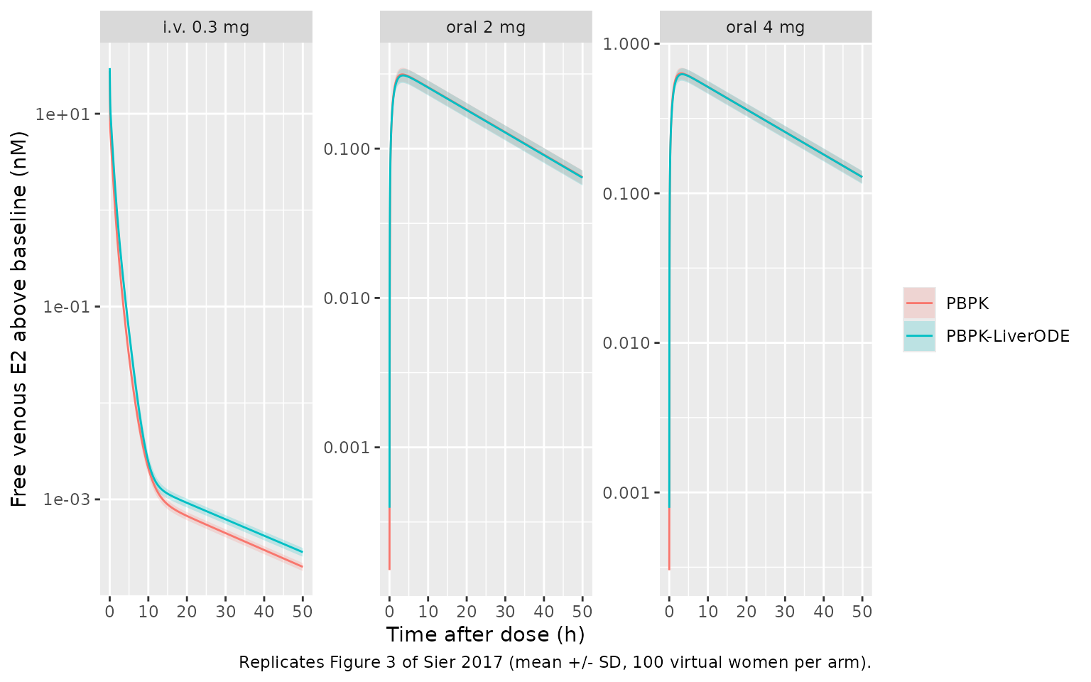
Figure 4: organ disposition after an i.v. bolus
The paper reports, for the reference simulation after the 0.3 mg i.v. bolus, organ Tmax from 0.1 h (kidney) to 0.93 h (adipose) for the base PBPK model, and a liver Cmax of 50.3 nM (PBPK) and 7.9 nM (PBPK-LiverODE).
organs <- c("lung", "adipose", "bone", "brain", "heart", "muscle", "skin",
            "intestine", "spleen", "stomach", "pancreas", "thymus", "kidney",
            "other", "vp_liver", "liver", "vp_gonads", "gonads")
ev_ref <- rxode2::et(amt = 1101, cmt = "depot_iv", time = 0) |>
  rxode2::et(sort(unique(c(seq(0, 2, by = 0.005), seq(2, 15, by = 0.05))))) |>
  as.data.frame() |>
  mutate(WT = 60, HT = 163, AGE = 35)
organ_tab <- lapply(names(models), function(nm) {
  s <- as.data.frame(rxode2::rxSolve(models[[nm]], ev_ref, atol = 1e-12, rtol = 1e-10))
  bind_rows(lapply(organs, function(o) {
    y <- s[[o]] - s[[o]][1]
    data.frame(model = nm, state = o, cmax = max(y), tmax = s$time[which.max(y)])
  }))
}) |> bind_rows()

organ_tab |>
  pivot_wider(names_from = model, values_from = c(cmax, tmax)) |>
  dplyr::rename(
    "State" = state,
    "PBPK Cmax (nM)" = cmax_PBPK, "PBPK Tmax (h)" = tmax_PBPK,
    "LiverODE Cmax (nM)" = `cmax_PBPK-LiverODE`, "LiverODE Tmax (h)" = `tmax_PBPK-LiverODE`
  ) |>
  knitr::kable(digits = 3, caption = paste(
    "Baseline-subtracted organ E2 after 0.3 mg i.v. in the reference woman",
    "(Figure 4a of Sier 2017)."
))| State | PBPK Cmax (nM) | LiverODE Cmax (nM) | PBPK Tmax (h) | LiverODE Tmax (h) |
|---|---|---|---|---|
| lung | 27.791 | 29.850 | 0.015 | 0.020 |
| adipose | 4.293 | 3.968 | 0.950 | 0.965 |
| bone | 7.552 | 4.598 | 0.580 | 0.865 |
| brain | 15.229 | 12.348 | 0.175 | 0.220 |
| heart | 16.668 | 13.123 | 0.130 | 0.170 |
| muscle | 6.311 | 5.379 | 0.695 | 0.755 |
| skin | 11.832 | 8.869 | 0.305 | 0.425 |
| intestine | 16.434 | 13.009 | 0.140 | 0.180 |
| spleen | 16.844 | 13.190 | 0.125 | 0.165 |
| stomach | 14.556 | 11.906 | 0.195 | 0.245 |
| pancreas | 14.986 | 12.182 | 0.185 | 0.230 |
| thymus | 13.553 | 11.246 | 0.235 | 0.280 |
| kidney | 16.609 | 12.819 | 0.100 | 0.145 |
| other | 13.605 | 11.283 | 0.230 | 0.275 |
| vp_liver | 15.447 | 7.908 | 0.190 | 0.190 |
| liver | 51.062 | 0.003 | 0.195 | 0.190 |
| vp_gonads | 0.445 | 0.385 | 2.850 | 3.000 |
| gonads | 4.447 | 3.854 | 2.850 | 3.000 |
pick <- function(m, s, col) organ_tab[[col]][organ_tab$model == m & organ_tab$state == s]
stopifnot(
  abs(pick("PBPK", "kidney", "tmax") - 0.1) < 0.05,
  abs(pick("PBPK", "adipose", "tmax") - 0.93) < 0.15,
  # Liver Cmax: the PBPK value is the hepatocyte state, the LiverODE value the
  # liver vascular state (see Assumptions and deviations).
  abs(pick("PBPK", "liver", "cmax") / 50.3 - 1) < 0.1,
  abs(pick("PBPK-LiverODE", "vp_liver", "cmax") / 7.9 - 1) < 0.1
)
PKNCA validation
Table 1 of the paper reports Cmax, Tmax and AUC as the mean +/- SD
over the virtual population. Its AUC column is headed “AUC-infinity”,
but the values match the AUC over the 50 h window of the Lyrenas study,
which is what is computed here (auclast over 0-50 h after
the dose).
sim_nca <- sim_exo |>
  dplyr::filter(!is.na(Cc_exo)) |>
  transmute(id, model, arm, time = tad, Cc = Cc_exo)
# The dose-time row (tad = 0, Cc = 0 above baseline) is in the grid already.
stopifnot(all(tapply(sim_nca$time, sim_nca$id, min) == 0))

dose_df <- events |>
  filter(evid == 1) |>
  transmute(id, arm, time = 0, amt) |>
  tidyr::crossing(model = names(models))

conc_obj <- PKNCA::PKNCAconc(sim_nca, Cc ~ time | model + arm + id)
dose_obj <- PKNCA::PKNCAdose(dose_df, amt ~ time | model + arm + id)
intervals <- data.frame(start = 0, end = 50, cmax = TRUE, tmax = TRUE, auclast = TRUE)
nca_res <- PKNCA::pk.nca(PKNCA::PKNCAdata(conc_obj, dose_obj, intervals = intervals))
Comparison against Table 1
published <- tibble::tribble(
  ~model,          ~arm,        ~cmax, ~tmax, ~auclast,
  "PBPK",          "i.v. 0.3 mg",    NA,    NA,     10.4,
  "PBPK",          "oral 2 mg",    0.34,   2.5,      8.9,
  "PBPK",          "oral 4 mg",    0.67,   3.1,     17.3,
  "PBPK-LiverODE", "i.v. 0.3 mg",    NA,    NA,      6.1,
  "PBPK-LiverODE", "oral 2 mg",    0.35,   3.5,      9.2,
  "PBPK-LiverODE", "oral 4 mg",    0.71,   3.2,     17.4
)
cmp <- nlmixr2lib::ncaComparisonTable(
  simulated = nca_res,
  reference = published,
  by = c("model", "arm"),
  units = c(cmax = "nM", tmax = "h", auclast = "nM*h"),
  tolerance_pct = 20
)
# Table 1 gives no Cmax or Tmax for the i.v. bolus; keep the rows it does report.
cmp <- cmp[grepl("[0-9]", cmp$Reference), ]
knitr::kable(cmp, caption = paste(
  "Simulated (median of 100 virtual women per arm) vs Table 1 of Sier 2017",
  "(mean of 1495). * differs from the published value by more than 20%."
))| NCA parameter | model | arm | Reference | Simulated | % diff | |
|---|---|---|---|---|---|---|
| 2 | Cmax (nM) | PBPK | oral 2 mg | 0.34 | 0.316 | -7.0% |
| 3 | Cmax (nM) | PBPK | oral 4 mg | 0.67 | 0.63 | -5.9% |
| 5 | Cmax (nM) | PBPK-LiverODE | oral 2 mg | 0.35 | 0.31 | -11.3% |
| 6 | Cmax (nM) | PBPK-LiverODE | oral 4 mg | 0.71 | 0.624 | -12.1% |
| 8 | Tmax (h) | PBPK | oral 2 mg | 2.5 | 3.3 | +32.0%* |
| 9 | Tmax (h) | PBPK | oral 4 mg | 3.1 | 3.1 | -0.0% |
| 11 | Tmax (h) | PBPK-LiverODE | oral 2 mg | 3.5 | 3.53 | +0.7% |
| 12 | Tmax (h) | PBPK-LiverODE | oral 4 mg | 3.2 | 3.35 | +4.7% |
| 13 | AUClast (nM*h) | PBPK | i.v. 0.3 mg | 10.4 | 6.53 | -37.2%* |
| 14 | AUClast (nM*h) | PBPK | oral 2 mg | 8.9 | 8.36 | -6.0% |
| 15 | AUClast (nM*h) | PBPK | oral 4 mg | 17.3 | 16.6 | -4.2% |
| 16 | AUClast (nM*h) | PBPK-LiverODE | i.v. 0.3 mg | 6.1 | 10.6 | +73.5%* |
| 17 | AUClast (nM*h) | PBPK-LiverODE | oral 2 mg | 9.2 | 8.27 | -10.1% |
| 18 | AUClast (nM*h) | PBPK-LiverODE | oral 4 mg | 17.4 | 16.5 | -4.9% |
sim_med <- as.data.frame(nca_res$result) |>
  group_by(model, arm, PPTESTCD) |>
  summarise(value = median(PPORRES), .groups = "drop") |>
  pivot_wider(names_from = PPTESTCD, values_from = value) |>
  left_join(published, by = c("model", "arm"), suffix = c("_sim", "_pub"))
oral <- sim_med |> filter(arm != "i.v. 0.3 mg")
stopifnot(
  # Oral arm: a mis-transcribed flow, volume, rate constant or dose moves
  # Cmax and AUC by tens of percent. Observed differences are -4% to -12%
  # (cohort median against the paper's mean); the model is deterministic and
  # the cohort comes from R's own RNG, so these do not vary between machines.
  all(abs(oral$cmax_sim / oral$cmax_pub - 1) < 0.2),
  all(abs(oral$auclast_sim / oral$auclast_pub - 1) < 0.2)
)
The oral arm reproduces Table 1 for both models, with differences of 4-12%. The i.v. AUC does not, in opposite directions for the two models; this is discussed below and is deliberately left out of the gate above. Simulated oral Tmax is later than the published base-PBPK value for the 2 mg dose; the published Tmax values are means over individual Tmax values on the paper’s own sampling grid, which is not reported.
Assumptions and deviations
- PBPK-GSMN is not packaged. Its hepatic clearance is a flux-balance linear programme over the Recon2 network (7440 reactions), re-solved at every step inside MuFINS through a quasi-steady-state Petri net. That is not an ODE system and cannot be expressed in rxode2. The phenytoin drug-drug interaction analysis (Figures 5-7) runs only on that model and is likewise out of scope.
- Observation is free venous E2. The paper does not say which venous quantity Table 1 and Figure 3 report. Free (unbound) E2 reproduces the published oral Cmax and AUC (within 2.5% for the base model’s reference woman); total E2 is about 57-fold higher. Values are baseline-subtracted, matching the radiolabelled-dose clinical comparators.
-
The deposits are the source of truth where they differ from
Additional file 1, because they are the authors’ executable
models and they reproduce the published results. For the base PBPK model
the maintainers confirmed that all 40 derived physiological quantities
(17 organ volumes, 15 blood flows, cardiac output, BSA, BMI, liver
weight, intrinsic clearance) computed from the equations in the model
file equal the deposited values to within 3e-13 relative error. The
differences are:
- E2 biosynthesis rate constant: deposit 2; Additional file 1 v17 prints 5. At steady state the gonad efflux flux is exactly -2.0000 nM/h, which only a +2 input balances; the BioModels curator note also gives 2.
- Skin volume: deposit
2.71^(1.63*BSA - 1.93)/1.5; the supplement printse^(2.63*ln(Height) - 1.93)/1.5, which gives 0.52 kg of skin instead of 2.11 kg. - Stomach volume density: deposit 1.044; the supplement prints 1.44.
- Cardiac output: deposit sums the 15 arterial-side organ flows; the supplement’s sum over i other than 8 and 10 counts the intestine twice.
- Gonad estrogen-receptor binding: deposit 3600 / 900 (as for the liver); Additional file 1 v18 prints 1000 / 100, which duplicates the permeability constants of v19.
- The deposits hard-code 2.718 and 2.71 in place of e; both literals are kept because they are needed to reproduce the deposited volumes.
- The base deposit delivers the i.v. dose at 1000 1/h; the main text, Additional file 1 and the BioModels curator note all give 250 1/h, which is used. AUC is unaffected.
- PBPK-LiverODE differs from the base PBPK beyond its liver. Its deposit computes blood flows without the tissue-density factor, sets lung flow to 0.55 x cardiac output, uses 46 nM of hepatic estrogen receptor and liver permeability constants of 150 / 41.7 1/h (the last stated in the main text). The maintainers checked the alternative of the base model’s flows: it halves the oral AUC (4.9 against the published 9.2 nM*h), so the deposited flows are the published model.
- LiverODE kinetic constants match the in vitro LiverODE reaction table of Additional file 1 except for four: CYP1A2 estrone 2-hydroxylation Km (deposit 19000 nM, table 1900), SULT1E1 and ABCG2-E13S kcat (deposit 150 and 8.46e6, table 8.46e6 and 150, i.e. swapped), MDR1 E2-17-glucuronide Km (deposit 62000, table 6200) and non-specific binding (deposit 3600 / 85500, table 0.1 / 0.1). Substituting the table value for the CYP1A2 Km, the SULT1E1 kcat or the binding constants, one at a time, changes no Table 1 metric at four significant figures, because the estrone branch and the binding pool do not feed back appreciably on E2; the two transporter constants act only on conjugates that have no path back to E2. Deposit values are used. The terminal metabolites (methoxy estrogens, glucuronides and sulfates once formed or exported) are fixed sinks in the deposit and are not carried as states.
- i.v. AUC. The simulated i.v. AUC is 7.1 nMh (PBPK) and 11.5 nMh (PBPK-LiverODE) for the reference woman, against 10.4 and 6.1 in Table 1; the oral arm of the same models matches. For the base model the maintainers ruled out the bolus rate, the integration grid, the AUC window, baseline handling and body-size effects (the cohort above spreads it only modestly). The paper’s own discussion of Figure 3a attributes the base model’s larger RMSE to “under prediction at higher concentrations in the base PBPK model”, which agrees with the simulated ordering here and not with Table 1; the two i.v. values in Table 1 may have been transposed. No parameter was adjusted.
- Plasma binding constants. The Results text says the Sodergard 1982 dissociation constants (23.8 uM albumin, 3.18 nM SHBG) replaced the Plowchalk and Teeguarden values. Both deposits and Additional file 1 use the Plowchalk and Teeguarden values (17 uM, 1.5 nM: koff/kon = 6.12e7/3600 and 5400/3600), and those, with 40 nM SHBG and 500 uM albumin, give the 52% / 46% split the paper reports. The deposited values are used.
- Baseline E2. Additional file 1 says the biosynthesis rate was fitted to 0.15 nM total (about 0.003 nM free) venous E2. The deposited steady state is 0.73 nM total / 0.013 nM free (PBPK) and 1.19 / 0.021 nM (PBPK-LiverODE). The deposited values are kept; the comparisons above are baseline-subtracted.
- Figure 4 liver and gonads. The published liver Cmax (50.3 nM PBPK, 7.9 nM PBPK-LiverODE) is reproduced by the hepatocyte state in the base model but by the liver vascular state in the LiverODE model (its hepatocyte free E2 peaks near 0.003 nM because the metabolism network clears it so fast). The gonad-to-plasma ratios at 1 h (49.7 and 21.3) were not reproduced under the free, total or baseline-subtracted definitions the maintainers tried; the closest, free gonad-cell over free venous E2, is about 25 and 15.
-
Virtual cohort. NHANES summary statistics were
digitised from Figure S7; weight, height and age are drawn
independently. The comparison uses the cohort median
(
ncaComparisonTable()aggregates by median) against the paper’s mean. -
Compartment names. The maintainers ratified the
bare organ names
thymusandgonads(the paper’s lumped uterus + ovaries) withvp_gonadsfor its vascular sub-compartment, location-suffixed plasma-protein states (shbg_venous,complex_albumin_arterial, …), receptor-named estrogen-receptor states (target_er_liver,complex_er_gonads, …), and thedepot_ivi.v. input compartment. The hepatocyte species of the LiverODE network are specific to this model and are declared as paper-specific compartments. - No erratum for the article was found (checked 2026-10-15).