Meropenem in preterm newborns (Zyryanov 2023)
Source:vignettes/articles/Zyryanov_2023_meropenem.Rmd
Zyryanov_2023_meropenem.RmdModel and source
- Citation: Zyryanov S, Bondareva I, Butranova O, Kazanova A. Population PK/PD modelling of meropenem in preterm newborns based on therapeutic drug monitoring data. Front Pharmacol. 2023;14:1079680. doi:10.3389/fphar.2023.1079680
- Description: One-compartment IV population PK model for meropenem in 66 preterm newborns in a Moscow neonatal intensive care unit, fitted to peak-trough therapeutic drug monitoring data (Zyryanov 2023). Pmetrics NPAG non-parametric fit parameterised by an elimination rate constant and an absolute volume of distribution, with zero-order (infusion) input and no covariates in the model: gestational, postnatal and postconceptual age, body weight and Schwartz GFR were related to the individual Bayesian estimates by univariate regression only, and no coefficients were reported. The NPAG joint density is approximated by independent log-normal marginals at the published medians and CV%. The assay-error polynomial used for weighting was not reported, so residual error is carried as fixed zero.
- Article: https://doi.org/10.3389/fphar.2023.1079680 (open access)
Population
Zyryanov 2023 retrospectively analysed routine therapeutic drug monitoring (TDM) of meropenem in 66 preterm newborns treated in the intensive care unit of City Clinical Hospital 24, Moscow, between January 2018 and February 2022. Each patient contributed one TDM occasion: a peak within 30 min after dosing and a trough just before the next dose (132 concentrations, HPLC-UV, LLOQ 0.2 mg/L). Meropenem was given empirically at 40-120 mg/kg/day as 1-3 h IV infusions two or three times a day (20-40 mg/kg per dose every 8-12 h); the daily dose at TDM was 94.6 +/- 40.4 mg/day.
Table 1 (mean +/- SD, median): gestational age 28.9 +/- 2.93 weeks (28.5), postnatal age at TDM 33.0 +/- 20.88 days (30.5), postconceptual age 33.6 +/- 3.69 weeks (33.6), weight 1.66 +/- 0.464 kg (1.58, IQR 1.30-2.04), height 38.3 +/- 4.26 cm, serum creatinine 46.66 +/- 20.235 umol/L, Schwartz GFR 27.31 +/- 9.676 mL/min/1.73 m^2; 39.4% female. Diagnoses included pneumonia (84.8%), necrotizing enterocolitis (60.6%) and bacterial meningitis (9.1%).
The same information is available programmatically via
readModelDb("Zyryanov_2023_meropenem")$population.
Source trace
Per-parameter origins are also recorded inline in
inst/modeldb/specificDrugs/Zyryanov_2023_meropenem.R.
| Equation / parameter | Value | Source location |
|---|---|---|
| Structure: one compartment, zero-order input, first-order elimination, parameterised by Kel and V | – | Methods, ‘PK analysis’ |
cl = kel * vc, t1/2 = 0.693 / kel
(derived) |
– | Methods, ‘PK analysis’ |
lkel |
log(0.30) 1/h | Results and Abstract: Kel 0.31 +/- 0.13 (median 0.3) |
lvc |
log(1.2) L | Results and Abstract: V 1.2 +/- 0.4 (median 1.2) |
etalkel |
log(0.42^2 + 1) = 0.1624 | Results: Kel CV 42% |
etalvc |
log(0.33^2 + 1) = 0.1033 | Results: V CV 33% |
propSd, addSd
|
fixed(0) | Methods: weighting by the inverse assay variance; coefficients not reported |
| Unbound fraction for PK/PD targets | 0.98 | Methods, ‘PD analysis’ |
| Derived medians used as checks | T1/2 2.33 h, CL 0.355 L/h, V 0.76 L/kg, CL 0.219 L/h/kg | Table 2 |
Typical-value check against Table 2
Table 2 summarises the individual Bayesian posterior half-lives and clearances. Their medians follow directly from the median Kel and V, which is why the medians (rather than the means 0.31 1/h and 1.2 L) are the typical values in the model file. Weight-normalised values use the Table 1 median weight of 1.58 kg.
mod <- readModelDb("Zyryanov_2023_meropenem")
ini_df <- rxode2::rxode(mod)$iniDf
#> ℹ parameter labels from comments will be replaced by 'label()'
theta <- setNames(ini_df$est, ini_df$name)
kel_tv <- exp(theta[["lkel"]])
v_tv <- exp(theta[["lvc"]])
wt_med <- 1.58

typical <- tibble::tibble(
  Quantity = c("T1/2 (h)", "CL (L/h)", "V (L/kg)", "CL (L/h/kg)"),
  Model = c(log(2) / kel_tv, kel_tv * v_tv, v_tv / wt_med, kel_tv * v_tv / wt_med),
  `Table 2 median` = c(2.33, 0.355, 0.76, 0.219)
) |>
  dplyr::mutate(`% diff` = round(100 * (Model / `Table 2 median` - 1), 1))
knitr::kable(typical, digits = 3)| Quantity | Model | Table 2 median | % diff |
|---|---|---|---|
| T1/2 (h) | 2.310 | 2.330 | -0.8 |
| CL (L/h) | 0.360 | 0.355 | 1.4 |
| V (L/kg) | 0.759 | 0.760 | -0.1 |
| CL (L/h/kg) | 0.228 | 0.219 | 4.0 |
Virtual cohort
The paper’s patients received a mix of regimens that is not tabulated per patient, so the simulation covers the corners of the reported range: 20 or 40 mg/kg per dose every 8 or 12 h as a 1-h infusion, plus 20 mg/kg every 8 h as a 3-h infusion (the longest infusion used). Weight is drawn log-normally around the Table 1 median of 1.58 kg with a spread matching its interquartile range. The model has no covariates, so weight affects only the mg dose. Dosing runs for 48 h; with a half-life of about 2.3 h the last dosing interval is at steady state.
rxode2::rxSetSeed(20230315)
n_per_arm <- 200

arms <- tibble::tibble(
  treatment = c(
    "20 mg/kg q12h (1 h)", "20 mg/kg q8h (1 h)", "20 mg/kg q8h (3 h)",
    "40 mg/kg q12h (1 h)", "40 mg/kg q8h (1 h)"
  ),
  mgkg = c(20, 20, 20, 40, 40),
  tau_h = c(12, 8, 8, 12, 8),
  inf_h = c(1, 1, 3, 1, 1)
)

subjects <- arms[rep(seq_len(nrow(arms)), each = n_per_arm), ] |>
  dplyr::mutate(
    id = dplyr::row_number(),
    WT = 1.58 * exp(stats::rnorm(dplyr::n(), 0, log(2.04 / 1.30) / 1.349))
  )

t_end <- 48
doses <- subjects |>
  dplyr::rowwise() |>
  dplyr::reframe(
    id = id,
    time = seq(0, t_end - tau_h, by = tau_h),
    amt = mgkg * WT,
    rate = mgkg * WT / inf_h
  ) |>
  dplyr::mutate(evid = 1L, cmt = "central")

obs <- tidyr::expand_grid(id = subjects$id, time = seq(0, t_end, by = 0.1)) |>
  dplyr::mutate(amt = NA_real_, rate = NA_real_, evid = 0L, cmt = "central")

events <- dplyr::bind_rows(doses, obs) |>
  dplyr::left_join(dplyr::select(subjects, id, treatment, tau_h, inf_h, WT), by = "id") |>
  dplyr::arrange(id, time, dplyr::desc(evid))
Simulation
sim <- rxode2::rxSolve(mod, events, keep = c("treatment", "tau_h", "inf_h", "WT")) |>
  as.data.frame()
#> ℹ parameter labels from comments will be replaced by 'label()'

# Last dosing interval (steady state) for every subject.
last_int <- sim |>
  dplyr::filter(time >= t_end - tau_h - 1e-8) |>
  dplyr::mutate(tad = time - (t_end - tau_h))
last_int |>
  dplyr::group_by(treatment, tad) |>
  dplyr::summarise(
    med = stats::median(Cc),
    lo = stats::quantile(Cc, 0.05),
    hi = stats::quantile(Cc, 0.95),
    .groups = "drop"
  ) |>
  ggplot(aes(tad, med)) +
  geom_ribbon(aes(ymin = lo, ymax = hi), alpha = 0.25) +
  geom_line() +
  geom_hline(yintercept = c(2, 8), linetype = "dashed") +
  facet_wrap(~treatment) +
  scale_y_log10() +
  labs(x = "Time after dose (h)", y = "Meropenem (mg/L)")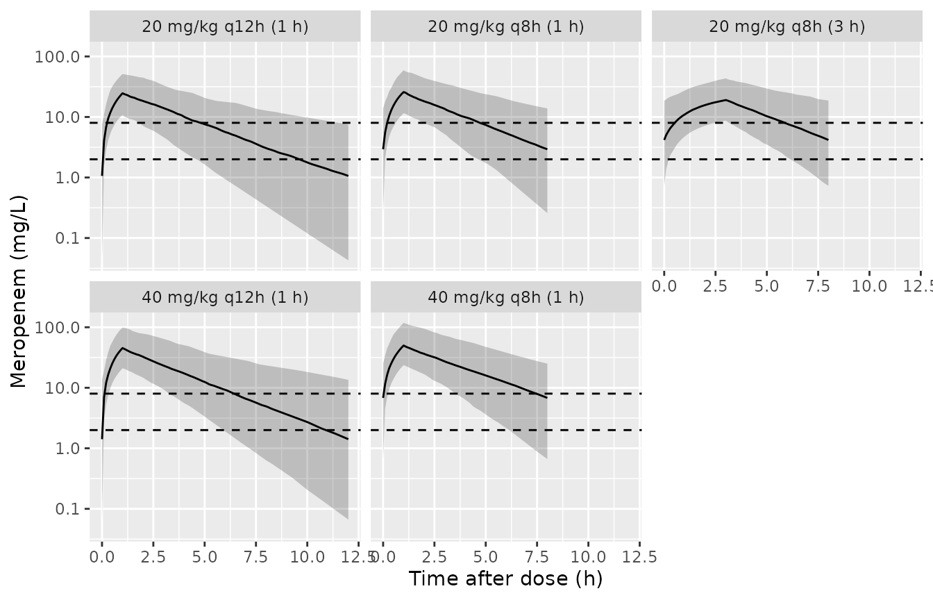
Simulated steady-state meropenem concentrations over the last dosing interval (median and 5th-95th percentiles) by regimen. Dashed lines mark the EUCAST susceptible (2 mg/L) and resistant (8 mg/L) breakpoints used by the paper.
Peaks and troughs against the TDM observations
The paper reports geometric means of 23.5 mg/L for peaks (sampled within 30 min after dosing) and 3.5 mg/L for troughs, pooled over all regimens. The cohort’s median daily dose at TDM, 94.3 mg/day at a median 1.58 kg, is about 60 mg/kg/day, which is the 20 mg/kg q8h regimen. The simulated peak is taken 15 min after the end of the infusion, the middle of the paper’s 30-min window.
pk_tr <- last_int |>
  dplyr::group_by(id, treatment) |>
  dplyr::summarise(
    peak = Cc[which.min(abs(tad - (inf_h[1] + 0.25)))],
    trough = Cc[which.max(tad)],
    .groups = "drop"
  )

gm_tab <- pk_tr |>
  dplyr::group_by(treatment) |>
  dplyr::summarise(
    `Peak GM (mg/L)` = exp(mean(log(peak))),
    `Trough GM (mg/L)` = exp(mean(log(trough))),
    `Trough <= 2 mg/L (%)` = 100 * mean(trough <= 2),
    `Trough < 4 mg/L (%)` = 100 * mean(trough < 4),
    `Trough > 8 mg/L (%)` = 100 * mean(trough > 8),
    .groups = "drop"
  )
obs_row <- tibble::tibble(
  treatment = "Observed TDM (all regimens)",
  `Peak GM (mg/L)` = 23.5,
  `Trough GM (mg/L)` = 3.5,
  `Trough <= 2 mg/L (%)` = 19.7,
  `Trough < 4 mg/L (%)` = 50,
  `Trough > 8 mg/L (%)` = 9.1
)
dplyr::bind_rows(gm_tab, obs_row) |>
  dplyr::rename(Regimen = treatment) |>
knitr::kable(digits = 1, caption = "Simulated steady-state peaks and troughs vs. the observed TDM summary (Results).")| Regimen | Peak GM (mg/L) | Trough GM (mg/L) | Trough <= 2 mg/L (%) | Trough < 4 mg/L (%) | Trough > 8 mg/L (%) |
|---|---|---|---|---|---|
| 20 mg/kg q12h (1 h) | 23.0 | 0.8 | 69.0 | 86.5 | 4.5 |
| 20 mg/kg q8h (1 h) | 23.9 | 2.7 | 34.0 | 60.0 | 16.5 |
| 20 mg/kg q8h (3 h) | 17.7 | 3.9 | 23.5 | 48.5 | 26.5 |
| 40 mg/kg q12h (1 h) | 43.1 | 1.2 | 55.5 | 72.0 | 11.5 |
| 40 mg/kg q8h (1 h) | 48.4 | 5.3 | 17.5 | 36.5 | 43.0 |
| Observed TDM (all regimens) | 23.5 | 3.5 | 19.7 | 50.0 | 9.1 |
ref_arm <- gm_tab |> dplyr::filter(treatment == "20 mg/kg q8h (1 h)")
# The observed values pool regimens that are not tabulated, so this is an
# envelope: a wrong volume, rate constant or unit moves the geometric means
# several-fold, well outside a factor of 1.5.
stopifnot(
  ref_arm$`Peak GM (mg/L)` / 23.5 > 1 / 1.5, ref_arm$`Peak GM (mg/L)` / 23.5 < 1.5,
  ref_arm$`Trough GM (mg/L)` / 3.5 > 1 / 1.5, ref_arm$`Trough GM (mg/L)` / 3.5 < 1.5
)
PKNCA validation
Steady-state NCA over the last dosing interval of each regimen. Table 2’s half-life median and the observed trough geometric mean are the only published exposure values; the trough reference is attached to the 20 mg/kg q8h regimen, which matches the cohort’s median daily dose.
# A 0.25-h grid is ample for the interval NCA and keeps PKNCA fast.
conc_df <- last_int |>
  dplyr::filter(abs(tad * 4 - round(tad * 4)) < 1e-6) |>
  dplyr::filter(!is.na(Cc)) |>
  dplyr::select(id, treatment, time, Cc)
dose_df <- doses |>
  dplyr::left_join(dplyr::select(subjects, id, treatment), by = "id") |>
  dplyr::select(id, treatment, time, amt)

conc_obj <- PKNCA::PKNCAconc(conc_df, Cc ~ time | treatment + id, concu = "mg/L", timeu = "h")
dose_obj <- PKNCA::PKNCAdose(dose_df, amt ~ time | treatment + id, doseu = "mg")

intervals <- arms |>
  dplyr::transmute(
    treatment,
    start = t_end - tau_h,
    end = t_end,
    cmax = TRUE,
    cmin = TRUE,
    auclast = TRUE,
    half.life = TRUE
  )

nca_res <- PKNCA::pk.nca(PKNCA::PKNCAdata(conc_obj, dose_obj, intervals = intervals))

published <- tibble::tibble(
  treatment = arms$treatment,
  half.life = 2.33,
  cmin = ifelse(arms$treatment == "20 mg/kg q8h (1 h)", 3.5, NA_real_)
)

cmp <- nlmixr2lib::ncaComparisonTable(
  simulated = nca_res,
  reference = published,
  by = "treatment",
  params = c("half.life", "cmin"),
  units = c(half.life = "h", cmin = "mg/L"),
  tolerance_pct = 20
)
knitr::kable(cmp, caption = "Simulated vs. published values. * differs from reference by >20%.")| NCA parameter | treatment | Reference | Simulated | % diff |
|---|---|---|---|---|
| Cmin (mg/L) | 20 mg/kg q12h (1 h) | — | 1.06 | — |
| Cmin (mg/L) | 20 mg/kg q8h (1 h) | 3.5 | 2.93 | -16.3% |
| Cmin (mg/L) | 20 mg/kg q8h (3 h) | — | 4.17 | — |
| Cmin (mg/L) | 40 mg/kg q12h (1 h) | — | 1.41 | — |
| Cmin (mg/L) | 40 mg/kg q8h (1 h) | — | 6.8 | — |
| t½ (h) | 20 mg/kg q12h (1 h) | 2.33 | 2.38 | +2.2% |
| t½ (h) | 20 mg/kg q8h (1 h) | 2.33 | 2.38 | +2.0% |
| t½ (h) | 20 mg/kg q8h (3 h) | 2.33 | 2.33 | -0.1% |
| t½ (h) | 40 mg/kg q12h (1 h) | 2.33 | 2.19 | -6.0% |
| t½ (h) | 40 mg/kg q8h (1 h) | 2.33 | 2.36 | +1.4% |
The simulated half-life reproduces the Table 2 median within a few percent in every regimen, as it must for a linear model; the residual difference is the terminal-phase point selection over a single dosing interval. The trough comparison is approximate: the observed 3.5 mg/L pools all regimens and infusion durations.
PK/PD target attainment (Figures 3 and 4)
The paper evaluated the fraction of the dosing interval with unbound concentration above the MIC (fT > MIC, unbound fraction 0.98) at MIC values of 1-32 mg/L, using each patient’s Bayesian posterior parameters and actual regimen, split by gestational age (< 32 vs >= 32 weeks). The population model has no covariates, so it cannot separate the two GA groups; the simulated regimens bracket them instead. Figure values below were read off the published bars and lines by the maintainers.
fu <- 0.98
mics <- c(1, 2, 4, 8, 16, 32)

ft <- last_int |>
  dplyr::select(id, treatment, tad, Cc) |>
  tidyr::crossing(MIC = mics) |>
  dplyr::group_by(id, treatment, MIC) |>
  dplyr::summarise(fT = 100 * mean(fu * Cc > MIC), .groups = "drop")

pta_sim <- ft |>
  dplyr::group_by(treatment, MIC) |>
  dplyr::summarise(
    `Median fT>MIC (%)` = stats::median(fT),
    `100% fT>MIC (% of patients)` = 100 * mean(fT >= 100),
    .groups = "drop"
  )

fig_ref <- tibble::tibble(
  MIC = mics,
  `Fig 3 median fT>MIC, GA < 32` = c(100, 100, 80, 52, 16, 0),
  `Fig 3 median fT>MIC, GA >= 32` = c(100, 100, 98, 68, 39, 0),
  `Fig 4 100% fT>MIC, GA < 32` = c(92, 75, 31, 8, 2, 0),
  `Fig 4 100% fT>MIC, GA >= 32` = c(100, 79, 57, 21, 7, 0)
)

pta_sim |>
  tidyr::pivot_wider(
    id_cols = MIC,
    names_from = treatment,
    values_from = `100% fT>MIC (% of patients)`
  ) |>
  dplyr::left_join(fig_ref |> dplyr::select(MIC, dplyr::starts_with("Fig 4")), by = "MIC") |>
knitr::kable(digits = 0, caption = "Percentage of patients with 100% fT > MIC: simulated regimens vs. Figure 4.")| MIC | 20 mg/kg q12h (1 h) | 20 mg/kg q8h (1 h) | 20 mg/kg q8h (3 h) | 40 mg/kg q12h (1 h) | 40 mg/kg q8h (1 h) | Fig 4 100% fT>MIC, GA < 32 | Fig 4 100% fT>MIC, GA >= 32 |
|---|---|---|---|---|---|---|---|
| 1 | 51 | 83 | 89 | 55 | 90 | 92 | 100 |
| 2 | 30 | 64 | 76 | 44 | 82 | 75 | 79 |
| 4 | 13 | 40 | 50 | 28 | 63 | 31 | 57 |
| 8 | 4 | 16 | 24 | 10 | 42 | 8 | 21 |
| 16 | 2 | 4 | 6 | 3 | 15 | 2 | 7 |
| 32 | 0 | 0 | 0 | 0 | 2 | 0 | 0 |
pta_sim |>
  tidyr::pivot_wider(
    id_cols = MIC,
    names_from = treatment,
    values_from = `Median fT>MIC (%)`
  ) |>
  dplyr::left_join(fig_ref |> dplyr::select(MIC, dplyr::starts_with("Fig 3")), by = "MIC") |>
knitr::kable(digits = 0, caption = "Median fT > MIC (%): simulated regimens vs. Figure 3.")| MIC | 20 mg/kg q12h (1 h) | 20 mg/kg q8h (1 h) | 20 mg/kg q8h (3 h) | 40 mg/kg q12h (1 h) | 40 mg/kg q8h (1 h) | Fig 3 median fT>MIC, GA < 32 | Fig 3 median fT>MIC, GA >= 32 |
|---|---|---|---|---|---|---|---|
| 1 | 100 | 100 | 100 | 100 | 100 | 100 | 100 |
| 2 | 79 | 100 | 100 | 89 | 100 | 100 | 100 |
| 4 | 58 | 84 | 100 | 71 | 100 | 80 | 98 |
| 8 | 36 | 55 | 65 | 52 | 90 | 52 | 68 |
| 16 | 15 | 22 | 18 | 32 | 57 | 16 | 39 |
| 32 | 0 | 0 | 0 | 11 | 22 | 0 | 0 |
fig4_long <- fig_ref |>
  dplyr::select(MIC, dplyr::starts_with("Fig 4")) |>
  tidyr::pivot_longer(-MIC, names_to = "group", values_to = "pct") |>
  dplyr::mutate(group = sub("Fig 4 100% fT>MIC, ", "Published ", group))

ggplot(pta_sim, aes(MIC, `100% fT>MIC (% of patients)`, colour = treatment)) +
  geom_line() +
  geom_point(data = fig4_long, aes(MIC, pct, shape = group), inherit.aes = FALSE, size = 2.5) +
  scale_x_log10(breaks = mics) +
  labs(x = "MIC (mg/L)", y = "Patients with 100% fT > MIC (%)", colour = "Simulated", shape = NULL)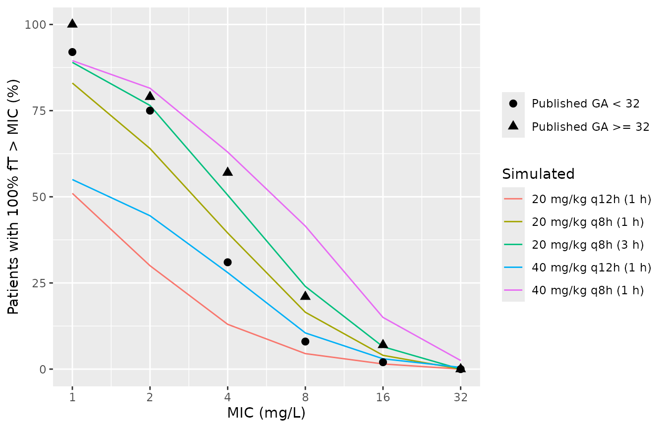
Replicates Figure 4 of Zyryanov 2023: percentage of patients achieving 100% fT > MIC. Lines are the simulated regimens; points are the published GA groups.
The published bars fall inside the band spanned by the simulated regimens at every MIC from 2 to 32 mg/L, as expected for a cohort treated with a mix of 20-40 mg/kg doses every 8-12 h. At 1 mg/L the published 92% and 100% sit at or just above the best simulated regimens (about 90%), whose log-normal tails include a few patients with a very short half-life. The Figure 3 medians for the younger group are close to the 20 mg/kg q8h 1-h regimen, the cohort’s median daily dose. The check below pins the band at the susceptible and resistant breakpoints.
band <- pta_sim |>
  dplyr::group_by(MIC) |>
  dplyr::summarise(
    lo = min(`100% fT>MIC (% of patients)`),
    hi = max(`100% fT>MIC (% of patients)`),
    .groups = "drop"
  ) |>
  dplyr::left_join(fig_ref, by = "MIC")
band_chk <- band |> dplyr::filter(MIC %in% c(2, 8))
# 10-point margin: the band edges are proportions from 200 simulated
# subjects, and the published bars are digitised group proportions.
stopifnot(
  all(band_chk$`Fig 4 100% fT>MIC, GA < 32` >= band_chk$lo - 10),
  all(band_chk$`Fig 4 100% fT>MIC, GA < 32` <= band_chk$hi + 10),
  all(band_chk$`Fig 4 100% fT>MIC, GA >= 32` >= band_chk$lo - 10),
  all(band_chk$`Fig 4 100% fT>MIC, GA >= 32` <= band_chk$hi + 10)
)
Assumptions and deviations
- Non-parametric density approximated by log-normal marginals. NPAG estimates a discrete joint distribution of support points (Figure 1 shows roughly 15 Kel and 15 V points). The model encodes independent log-normal marginals with the published medians and CV%; correlations between Kel and V are not reported and the multimodality visible in Figure 1 is not recoverable.
- Medians as typical values. The paper reports mean +/- SD (median) for Kel (0.31 +/- 0.13, median 0.3 1/h) and V (1.2 +/- 0.4, median 1.2 L). The medians are used because they reproduce the Table 2 derived medians (T1/2 2.33 h, CL 0.355 L/h); the mean Kel would change the typical value by 3%.
- Kel unit. The Results sentence prints the Kel unit as ‘L/h’; the Abstract’s ‘1/h’ is the correct unit for a rate constant and is used here.
-
Residual error not reported. Observations were
weighted by the inverse of the assay variance (a Pmetrics assay-error
polynomial), but neither its coefficients nor a gamma or lambda term are
given, and the article has no supplement. Both residual terms are
therefore
fixed(0); simulated concentrations are individual predictions without measurement noise. -
No covariates in the model. Body weight,
postconceptual age and Schwartz GFR were significant univariate
predictors of the individual half-life and volume, but the paper reports
no regression coefficients and states that multivariate analysis was not
performed. These are documented in
covariatesDataExcluded. Volume and clearance are absolute (L, L/h), so the model should be used only for patients resembling the 1.0-2.5 kg study cohort. - Regimens in the target-attainment comparison. Per-patient regimens are not published, so the Figure 3 and 4 comparisons use bracketing regimens rather than the paper’s patients, and the GA split cannot be reproduced.