Primaquine in lactating women and breastfed infants (Wattanakul 2024)
Source:vignettes/articles/Wattanakul_2024_primaquine_lactation.Rmd
Wattanakul_2024_primaquine_lactation.RmdModel and source
This paper contributes two model files. The first is the population PK model that was fitted to maternal data; the second extends it with a breastfed-infant compartment chain and was used only for simulation.
mother <- readModelDb("Wattanakul_2024_primaquine")
dyad <- readModelDb("Wattanakul_2024_primaquine_motherinfant")- Citation: Wattanakul T, Gilder ME, McGready R, Hanpithakpong W, Day NPJ, White NJ, Nosten F, Tarning J, Hoglund RM. Population pharmacokinetic modelling of primaquine exposures in lactating women and breastfed infants. Nat Commun. 2024;15:3851. doi:10.1038/s41467-024-47908-y. Parameter values taken from the NONMEM control stream in the Supplementary Information (‘NONMEM code’) and the identical Zenodo deposit doi:10.5281/zenodo.10925291 (‘Mother-to-infant.mod’), cross-checked against Table 2 of the main paper.
- Article: https://doi.org/10.1038/s41467-024-47908-y
- NONMEM control stream: Supplementary Information (“NONMEM code”), and the identical Zenodo deposit https://doi.org/10.5281/zenodo.10925291 (“Mother-to-infant.mod”).
Wattanakul_2024_primaquine – the
maternal model. Nine compartments: a four-transit absorption chain
feeding, by first-pass metabolism, either the primaquine or the
carboxyprimaquine central compartment, each of which exchanges with its
own breast-milk compartment. Six endpoints were fitted simultaneously:
each analyte in venous plasma, capillary plasma, and breast milk. This
is the model behind Table 2, Figure 2, and Table 3.
Wattanakul_2024_primaquine_motherinfant
– the mother-to-infant model. The same nine maternal compartments plus
eight infant compartments, and the breast-milk compartments are now
emptied into the infant at each feed. This is the model behind Figures 3
to 6. No infant parameter was estimated: all but one infant primaquine
sample was below the limit of quantification, so the infant layer is
entirely predictive.
All amounts in both models are molar (nmol, nmol/L), because the source paper fitted the natural logarithm of molar concentrations – the primaquine to carboxyprimaquine conversion is 1:1 molar, so a molar parameterisation makes the metabolite mass balance exact.
# Molecular weights of the free bases, used ONLY to convert model output
# (nmol/L) to the ng/mL units the paper reports. These are chemical
# constants, not model parameters, and are not stated in the paper --
# see "Assumptions and deviations".
MW_PQ  <- 259.35   # primaquine, C15H21N3O
MW_CPQ <- 274.32   # carboxyprimaquine, C15H18N2O3
Population
Twenty-one lactating women with a history of Plasmodium vivax infection and no previous primaquine radical-cure treatment were enrolled at three Shoklo Malaria Research Unit clinics on the Thai-Myanmar border between 11 November 2012 and 24 June 2014 (ClinicalTrials.gov NCT01780753). Median age was 23 years (18-40) and median body weight 51 kg (35-81). Each woman had one breastfeeding infant at least 28 days old: median age 0.42 years (0.13-1.81), median weight 6.8 kg (4.13-10.8), 14 male and 7 female. Both mother and infant were required to be G6PD-normal. Women reported a median of 11 breastfeeds per day (6-18) with a calculated infant daily milk intake of 1020 mL (619-1620). Baseline demographics are Table 1 of the source paper.
Each woman received primaquine 0.5 mg base/kg once daily for 14 days as directly observed oral therapy under non-fasting conditions. Venous plasma was sampled densely on days 0 and 13 and sparsely on days 3 and 7; capillary plasma at 0, 2, 6 and 12 h on days 0 and 13; breast milk by manual expression in the 1-3, 3-7, 7-12 and 12-24 h windows on days 0 and 13 plus one 1-3 h sample on days 3 and 7. The assay LLOQ was 1.14 ng/mL for primaquine and 4.88 ng/mL for carboxyprimaquine in every matrix.
The same information is available programmatically:
str(readModelDb("Wattanakul_2024_primaquine")()$population, max.level = 1)
#> Warning: some etas defaulted to non-mu referenced, possible parsing error: etaiov_fdepot_1, etaiov_fdepot_2, etaiov_fdepot_3, etaiov_fdepot_4, etaiov_mtt_1, etaiov_mtt_2, etaiov_mtt_3, etaiov_mtt_4
#> as a work-around try putting the mu-referenced expression on a simple line
#> List of 14
#>  $ species        : chr "human"
#>  $ n_subjects     : num 21
#>  $ n_studies      : num 1
#>  $ age_range      : chr "18-40 years"
#>  $ age_median     : chr "23 years"
#>  $ weight_range   : chr "35-81 kg"
#>  $ weight_median  : chr "51 kg"
#>  $ sex_female_pct : num 100
#>  $ disease_state  : chr "Lactating women with a history of Plasmodium vivax infection and no previous primaquine radical-cure treatment;"| __truncated__
#>  $ dose_range     : chr "Primaquine 0.5 mg base/kg once daily for 14 days, given orally under non-fasting conditions as directly observed therapy."
#>  $ regions        : chr "Thai-Myanmar border (three Shoklo Malaria Research Unit clinics), enrolled 11 November 2012 to 24 June 2014; Cl"| __truncated__
#>  $ infant_partner : chr "Each mother had one breastfeeding infant at least 28 days old: n = 21, age 0.42 years (0.13-1.81), weight 6.8 k"| __truncated__
#>  $ feeding_pattern: chr "Average 11 breastfeeds per day (6-18) and calculated infant daily milk intake 1020 mL (619-1620) per Table 1; t"| __truncated__
#>  $ notes          : chr "Baseline demographics from Wattanakul 2024 Table 1. Sampling: dense venous sampling on days 0 and 13 (0, 0.5, 1"| __truncated__
Source trace
Per-parameter origin is recorded as an in-file comment next to each
ini() entry in
inst/modeldb/specificDrugs/Wattanakul_2024_primaquine.R and
..._motherinfant.R. The table collects them here.
The control stream is a
$SIM (123456) ONLYSIM SUBPROBLEMS=1000 simulation deck. A
simulation deck carries final estimates by
construction, and this one is confirmed twice over: its twelve
$THETA entries equal Table 2’s population estimates
exactly, and back-computing
%CV = 100 * sqrt(exp(omega^2) - 1) – the formula Table 2
footnote a gives – reproduces Table 2’s IIV/IOV column to three
significant figures for nine of the ten random-effect terms.
| Equation / parameter | Value | Source location |
|---|---|---|
lfdepot (F) |
1 fixed | Table 2 “F 1 fixed”; $THETA 1 (1) FIX
|
lcl (CL/F PQ) |
17.1 L/h | Table 2; $THETA 2 |
lvc (V/F PQ) |
131 L | Table 2; $THETA 3 |
lcl_cpq (CL/F CPQ) |
0.967 L/h | Table 2; $THETA 4 |
lvc_cpq (V/F CPQ) |
22.7 L | Table 2; $THETA 5 |
lmtt (MTT) |
1.44 h | Table 2; $THETA 6 |
logitfm (FM) |
0.282 | Table 2; $THETA 7; logit transform in
$PK
|
lq_milk (Q/F) |
0.400 L/h, shared PQ/CPQ | Table 2 footnote c; $THETA 8; $PK
QCPQ=QPQ
|
pcmilk (PC PQ) |
0.376 | Table 2; $THETA 9 |
pcmilk_cpq (PC CPQ) |
0.00889 | Table 2; $THETA 10 |
cfcap (CF PQ) |
0.898 | Table 2; $THETA 11 |
cfcap_cpq (CF CPQ) |
1.06 | Table 2; $THETA 12 |
e_wt_cl, e_wt_vc
|
0.75, 1 fixed a priori | Methods; $PK (WT/51)**0.75,
(WT/51)
|
feed_n, feed_window,
feed_first
|
10/day, 0.4 h, 1 h | Results “Predicting infant concentrations”;
$PK/$DES
|
milk_intake |
0.15 L/kg/day | Eq. 1 (150 mL/kg infant body weight) |
kmilkinf (MTINF) |
100 /h fixed | Results; $PK MTINFPQ=MTINFCPQ=100
|
lmtt_infant |
0.706 h fixed | Methods, from a paediatric literature model (ref. 13);
$PK INFMTT
|
pma_tm50 |
7.6 months fixed | Eq. 4 and Methods (55% MAO-A activity at term birth);
$PK TM50
|
IIV etalfdepot … etalq_milk
|
0.0243 … 0.590 |
$OMEGA 1-8; cross-checked against Table 2 IIV
column |
IOV etaiov_fdepot_*, etaiov_mtt_*
|
0.0413, 0.280 |
$OMEGA 11-18 (BLOCK(1) +
SAME); Table 2 IOV column |
Residual expSd*
|
sqrt of 0.102, 0.0570, 0.0198, 0.0115, 0.156, 0.0911 | Table 2 sigma rows; $SIGMA 1-6 |
| Transit chain, first-pass split | n/a |
$DES DADT(1),
DADT(4)-DADT(7); $PK
K72=KTR*(1-FM), K73=KTR*FM
|
| Central / milk exchange | n/a |
$DES DADT(2), DADT(3),
DADT(8), DADT(9); $PK
K28, K82, K39,
K93
|
| Square-wave breastfeeding gate | n/a | Eqs. 5-8; $DES SQW1,
SQW2
|
| Milk-compartment volume | n/a | Eq. 1; $PK VMPQ=(0.15*INFWT)/FEEDNO
|
| Infant scaling, MAO-A maturation | n/a | Eq. 4; $PK INFCLP, INFV2,
INFCLM, INFV3, MF
|
| Infant compartment chain | n/a |
$DES DADT(10)-DADT(17)
|
Why the paper’s model is split into two files
The maternal model and the mother-to-infant model differ in exactly one term: whether the breast-milk compartments are drained by breastfeeding. That single term is load-bearing, and the paper’s own numbers identify which model produced which result.
At pseudo-equilibrium and with no drain, the milk:plasma
concentration ratio equals the partition coefficient
pcmilk exactly, so the milk:plasma AUC ratio must equal
0.376. Table 3 reports it as 0.376 (0.375-0.377) across every dosing
scenario. Simulating the same quantity with the drain present gives
about 0.28. Table 3 is therefore a maternal-model result – consistent
with its title, “simulated from the final pharmacokinetic model in the
breastfeeding mother” – and the drain belongs only to the
mother-to-infant model. This is verified numerically below.
Virtual cohort
Individual-level data are not public. The cohort below reproduces the published maternal weight range (35-81 kg, Table 1) and the study’s dosing regimen. Infant weight is fixed at the cohort median of 6.8 kg because in the maternal model it enters only through the breast-milk compartment volume.
set.seed(20240501)
N_MOTHERS <- 50L
T_END     <- 408      # 14 daily doses (0-312 h) + 72 h washout for half-life
GRID      <- 0.25

wt <- round(runif(N_MOTHERS, 35, 81), 1)

obs <- expand.grid(time = seq(0, T_END, by = GRID), id = seq_len(N_MOTHERS))
obs$evid <- 0L
obs$amt  <- NA_real_
# `cmt` on an observation row must name an ODE STATE, never an algebraic
# observable such as `Cc` -- rxode2 returns every observable as a column
# regardless of which state the row points at.
obs$cmt  <- "central"
obs$dvid <- 1L

dos <- expand.grid(time = seq(0, 13 * 24, by = 24), id = seq_len(N_MOTHERS))
dos$evid <- 1L
dos$cmt  <- "depot"
dos$dvid <- NA_integer_
dos$amt  <- (0.5 * wt[dos$id]) * 1e-3 / MW_PQ * 1e9   # 0.5 mg base/kg -> nmol

events <- rbind(
  obs[, c("id", "time", "evid", "amt", "cmt", "dvid")],
  dos[, c("id", "time", "evid", "amt", "cmt", "dvid")]
)
events <- events[order(events$id, events$time, -events$evid), ]
events$WT        <- wt[events$id]
events$WT_INFANT <- 6.8
events$OCC       <- 1L

summary(wt)
#>    Min. 1st Qu.  Median    Mean 3rd Qu.    Max.
#>   37.00   47.23   56.95   56.67   66.22   79.00
Simulation
sim <- rxode2::rxSolve(
  mother, events,
  # rxode2's ODE -> linCmt auto-conversion corrupts the dvid mapping for
  # multi-output models such as this one.
  useLinCmt = FALSE,
  atol = 1e-6, rtol = 1e-6,
  keep = c("WT")
) |>
  as.data.frame()
#> ℹ parameter labels from comments will be replaced by 'label()'
#> Warning: some etas defaulted to non-mu referenced, possible parsing error: etaiov_fdepot_1, etaiov_fdepot_2, etaiov_fdepot_3, etaiov_fdepot_4, etaiov_mtt_1, etaiov_mtt_2, etaiov_mtt_3, etaiov_mtt_4
#> as a work-around try putting the mu-referenced expression on a simple line

# rxSolve can silently drop subjects; assert the cohort survived.
stopifnot(length(unique(sim$id)) == N_MOTHERS)

sim <- sim |>
  mutate(
    `PQ plasma`     = Cc        * MW_PQ  / 1000,
    `PQ capillary`  = Ccap      * MW_PQ  / 1000,
    `PQ milk`       = Cmilk     * MW_PQ  / 1000,
    `CPQ plasma`    = Cc_cpq    * MW_CPQ / 1000,
    `CPQ capillary` = Ccap_cpq  * MW_CPQ / 1000,
    `CPQ milk`      = Cmilk_cpq * MW_CPQ / 1000
  )
nrow(sim)
#> [1] 81650
Replicate published figures
Figure 2 – prediction-corrected VPC of the six fitted endpoints
Figure 2 of Wattanakul 2024 shows the model’s predictive performance for primaquine and carboxyprimaquine in venous plasma, capillary plasma, and breast milk. Here the six endpoints are shown over the day-13 dosing interval, the occasion on which all three matrices were densely sampled.
# Replicates Figure 2 of Wattanakul 2024: median and 5th-95th percentile
# envelope of each fitted endpoint over the last (day 13) dosing interval.
vpc_levels <- c("PQ plasma", "PQ capillary", "PQ milk",
                "CPQ plasma", "CPQ capillary", "CPQ milk")

sim |>
  filter(time >= 312, time <= 336) |>
  mutate(tad = time - 312) |>
  select(id, tad, all_of(vpc_levels)) |>
  pivot_longer(all_of(vpc_levels), names_to = "endpoint", values_to = "conc") |>
  mutate(endpoint = factor(endpoint, levels = vpc_levels)) |>
  group_by(endpoint, tad) |>
  summarise(
    Q05 = quantile(conc, 0.05, na.rm = TRUE),
    Q50 = quantile(conc, 0.50, na.rm = TRUE),
    Q95 = quantile(conc, 0.95, na.rm = TRUE),
    .groups = "drop"
  ) |>
  ggplot(aes(tad, Q50)) +
  geom_ribbon(aes(ymin = Q05, ymax = Q95), alpha = 0.25) +
  geom_line() +
  facet_wrap(~endpoint, scales = "free_y", ncol = 3) +
  labs(
    x = "Time after the day-13 dose (h)", y = "Concentration (ng/mL)",
    title = "Figure 2 -- simulated median and 90% interval, six fitted endpoints",
    caption = "Replicates Figure 2 of Wattanakul 2024 (n = 50 virtual mothers)."
  ) +
  theme_bw()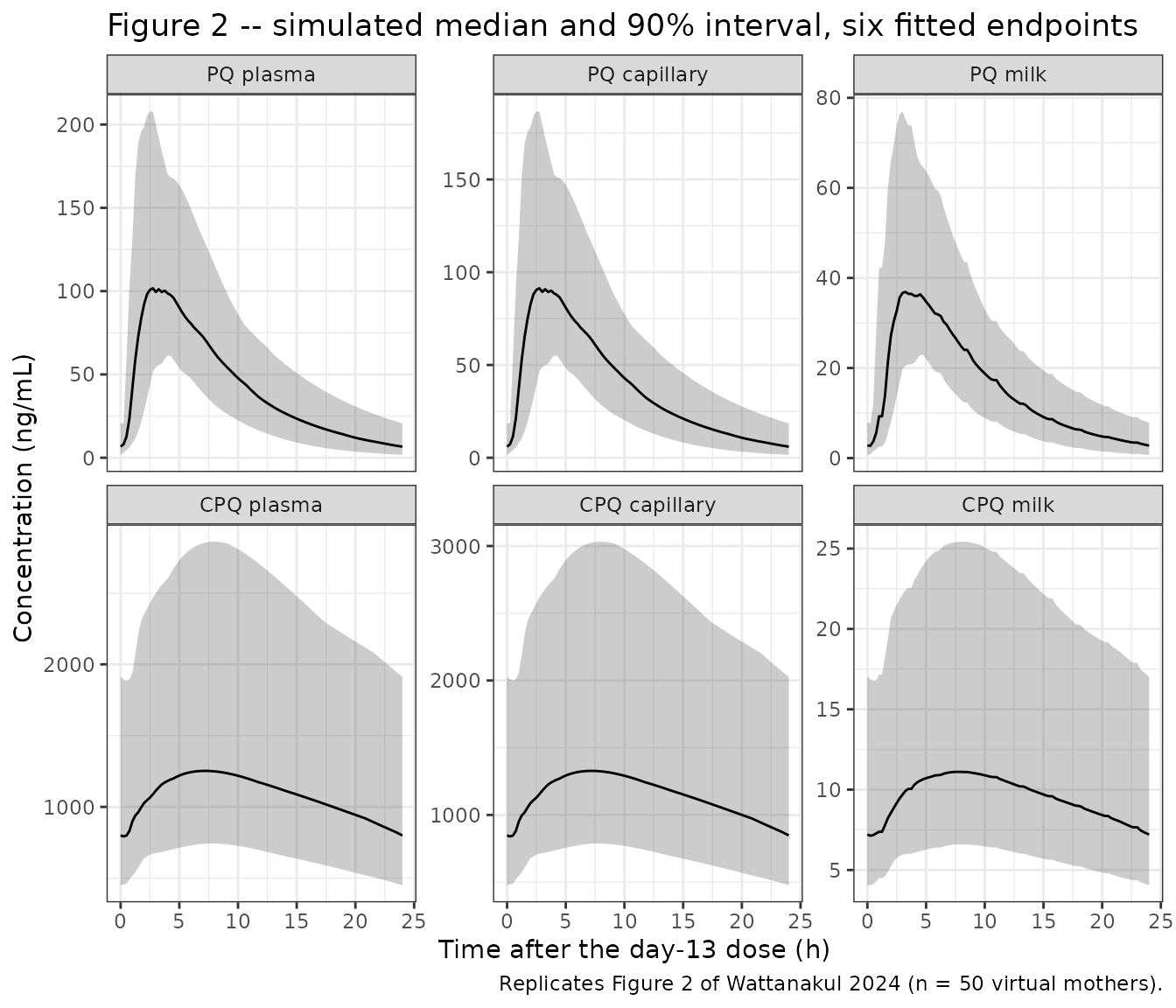
The visible flat steps in the two breast-milk panels are the square-wave gate: every 2.4 h the plasma-to-milk exchange closes for a 24-minute feeding window, during which the milk concentration is held constant.
The square-wave breastfeeding gate
The gate is worth showing on its own, because a transcription error in it would silently invert the feeding schedule. With 10 feeds/day the cycle is 2.4 h, the first feed starts at 1 h, and each feed lasts 0.4 h.
feed_n <- 10; feed_window <- 0.4; feed_first <- 1
cycle  <- 24 / feed_n
rest   <- cycle - feed_window
psh1   <- 4 * pi * (rest - feed_first) / cycle
per1   <- 2 * pi *  rest / cycle
tt     <- seq(0, 12, by = 0.002)
xw     <- sin(2 * pi * tt / cycle + (pi - per1 + psh1) / 2) - sin((pi - per1) / 2)
aw     <- sqrt(xw * xw + 1e-12)

data.frame(time = tt, sqwMilkToInfant = (aw - xw) / (2 * aw)) |>
  ggplot(aes(time, sqwMilkToInfant)) +
  geom_line() +
  scale_x_continuous(breaks = seq(0, 12, 1)) +
  labs(x = "Time (h)", y = "Gate open (1 = feeding)",
       title = "Equations 5-8: breastfeeding square wave",
       caption = "Feeds at 1.0-1.4, 3.4-3.8, 5.8-6.2 h ... (2.4 h cycle).") +
  theme_bw()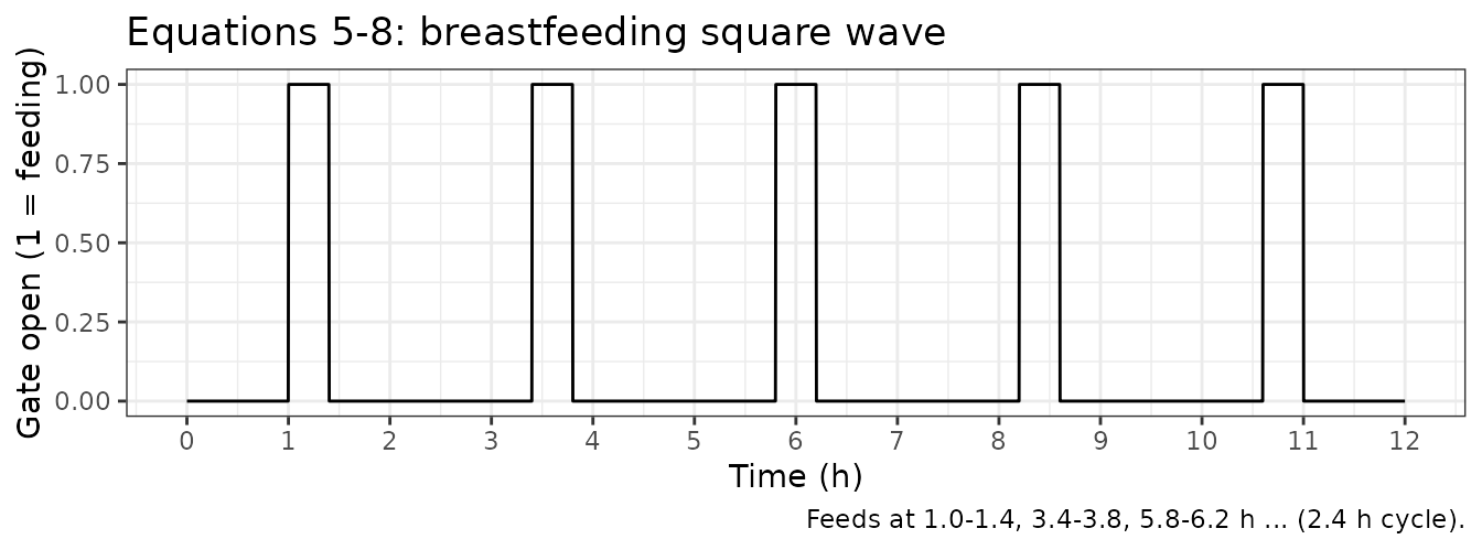
# The gate must be open for exactly feed_window hours per cycle, starting at
# feed_first. Assert it rather than eyeballing the figure.
open <- tt[(aw - xw) / (2 * aw) > 0.5]
stopifnot(
  abs(min(open) - feed_first) < 0.01,
  abs(diff(range(open[open < 2])) - feed_window) < 0.01
)
c(first_feed_start = min(open), duty_cycle = mean((aw - xw) / (2 * aw)))
#> first_feed_start       duty_cycle
#>        1.0000000        0.1666389
The duty cycle is feed_window / cycle = 0.4 / 2.4 =
0.1667, which the value above reproduces.
PKNCA validation
Table 2 of Wattanakul 2024 reports secondary NCA parameters for both analytes in plasma and in breast milk. AUC is over the whole 0-336 h treatment course; Cmax, Tmax and half-life are computed here over the final dosing interval and its washout.
analytes <- c("PQ plasma", "CPQ plasma", "PQ milk", "CPQ milk")

nca_long <- sim |>
  select(id, time, all_of(analytes)) |>
  pivot_longer(all_of(analytes), names_to = "analyte", values_to = "Cc") |>
  # Only drop missing values -- filtering on `time > 0` or `Cc > 0` would
  # discard the time-zero anchor PKNCA needs for AUC.
  filter(!is.na(Cc))

# Guarantee a time-zero record per (analyte, id); pre-dose Cc = 0 is correct
# for an extravascular first dose.
nca_long <- bind_rows(
  nca_long,
  nca_long |> distinct(analyte, id) |> mutate(time = 0, Cc = 0)
) |>
  distinct(analyte, id, time, .keep_all = TRUE) |>
  arrange(analyte, id, time)

dose_long <- events |>
  filter(evid == 1) |>
  select(id, time, amt) |>
  tidyr::crossing(analyte = analytes) |>
  arrange(analyte, id, time)
# AUC over the full 0-336 h course.
conc_auc <- PKNCA::PKNCAconc(
  nca_long |> filter(time <= 336),
  Cc ~ time | analyte + id
)
dose_auc <- PKNCA::PKNCAdose(dose_long, amt ~ time | analyte + id)

res_auc <- PKNCA::pk.nca(PKNCA::PKNCAdata(
  conc_auc, dose_auc,
  intervals = data.frame(start = 0, end = 336, auclast = TRUE)
))
# Cmax / Tmax / half-life over the final dosing interval, with time rebased so
# that the day-13 dose is at t = 0 (Tmax is then time after dose, directly
# comparable with the paper).
conc_last <- PKNCA::PKNCAconc(
  nca_long |> filter(time >= 312) |> mutate(time = time - 312),
  Cc ~ time | analyte + id
)
dose_last <- PKNCA::PKNCAdose(
  dose_long |> filter(time == 312) |> mutate(time = 0),
  amt ~ time | analyte + id
)

res_last <- PKNCA::pk.nca(PKNCA::PKNCAdata(
  conc_last, dose_last,
  intervals = data.frame(
    start     = c(0, 0),
    end       = c(24, Inf),
    cmax      = c(TRUE,  FALSE),
    tmax      = c(TRUE,  FALSE),
    half.life = c(FALSE, TRUE)
  )
))
simulated <- bind_rows(
  as.data.frame(res_auc$result),
  as.data.frame(res_last$result)
) |>
  filter(PPTESTCD %in% c("auclast", "cmax", "tmax", "half.life")) |>
  # AUC: ng*h/mL -> ug*h/mL, matching the paper's units.
  mutate(PPORRES = if_else(PPTESTCD == "auclast", PPORRES / 1000, PPORRES)) |>
  select(analyte, PPTESTCD, PPORRES)
Comparison against published NCA
# Wattanakul 2024 Table 2, "Secondary pharmacokinetic parameters", median
# (min-max) across the 21 women. Breast-milk half-life is not reported.
published <- tibble::tribble(
  ~analyte,     ~PPTESTCD,   ~PPORRES,
  "PQ plasma",  "tmax",         2.80,
  "PQ plasma",  "cmax",       120,
  "PQ plasma",  "auclast",     14.3,
  "PQ plasma",  "half.life",    4.95,
  "CPQ plasma", "tmax",         6.78,
  "CPQ plasma", "cmax",      1255,
  "CPQ plasma", "auclast",    349,
  "CPQ plasma", "half.life",   17.2,
  "PQ milk",    "tmax",         3.43,
  "PQ milk",    "cmax",        44.7,
  "PQ milk",    "auclast",      5.38,
  "CPQ milk",   "tmax",         7.67,
  "CPQ milk",   "cmax",        11.2,
  "CPQ milk",   "auclast",      3.10
)

cmp <- nlmixr2lib::ncaComparisonTable(
  simulated     = simulated,
  reference     = published,
  by            = "analyte",
  units         = c(cmax = "ng/mL", auclast = "ug*h/mL",
                    tmax = "h", half.life = "h"),
  tolerance_pct = 20
)

knitr::kable(
  cmp,
  caption = paste(
    "Simulated (n = 50 virtual mothers, median) vs. Wattanakul 2024 Table 2",
    "secondary NCA parameters (n = 21, median). * differs by >20%."
  ),
  align = c("l", "l", "r", "r", "r")
)| NCA parameter | analyte | Reference | Simulated | % diff |
|---|---|---|---|---|
| Cmax (ng/mL) | PQ plasma | 120 | 114 | -5.4% |
| Cmax (ng/mL) | CPQ plasma | 1260 | 1250 | -0.2% |
| Cmax (ng/mL) | PQ milk | 44.7 | 42.1 | -5.8% |
| Cmax (ng/mL) | CPQ milk | 11.2 | 11.1 | -0.7% |
| Tmax (h) | PQ plasma | 2.8 | 2.88 | +2.7% |
| Tmax (h) | CPQ plasma | 6.78 | 7 | +3.2% |
| Tmax (h) | PQ milk | 3.43 | 3.25 | -5.2% |
| Tmax (h) | CPQ milk | 7.67 | 7.5 | -2.2% |
| AUClast (ug*h/mL) | PQ plasma | 14.3 | 14.2 | -0.9% |
| AUClast (ug*h/mL) | CPQ plasma | 349 | 338 | -3.1% |
| AUClast (ug*h/mL) | PQ milk | 5.38 | 5.33 | -0.9% |
| AUClast (ug*h/mL) | CPQ milk | 3.1 | 3 | -3.1% |
| t½ (h) | PQ plasma | 4.95 | 4.84 | -2.3% |
| t½ (h) | CPQ plasma | 17.2 | 15.9 | -7.4% |
Every parameter agrees with the published median. This is a meaningful check rather than a tautology: none of these fourteen numbers is a model parameter. They emerge from the whole system – the transit chain, the first-pass split, the formation-limited metabolite disposition, the milk partition, and the molar-to-mass conversion – so a sign error or a misread scale in any of them would show up here.
Table 3 – infant dose delivered through breast milk
Table 3 reports, for four maternal dosing scenarios, the milk:plasma AUC ratio, the total daily primaquine dose the infant receives, and that dose relative to the mother’s weight-adjusted dose. All three come from the maternal model.
scenarios <- tibble::tribble(
  ~scenario,                       ~mgkg, ~ii, ~ndose,
  "0.5 mg/kg OD x 14 d (standard)",  0.5,  24,     14,
  "1 mg/kg OD x 7 d (high)",         1.0,  24,      7,
  "0.5 mg/kg BID x 7 d (high)",      0.5,  12,     14,
  "0.25 mg/kg single (low)",         0.25, 24,      1
)

WT_M <- 51; WT_I <- 6.8

make_scenario <- function(i, id) {
  s  <- scenarios[i, ]
  dt <- seq(0, (s$ndose - 1) * s$ii, by = s$ii)
  last_dose <- max(dt)
  o <- data.frame(time = seq(0, last_dose + 24, by = 0.05),
                  evid = 0L, amt = NA_real_, cmt = "central", dvid = 1L)
  d <- data.frame(time = dt, evid = 1L,
                  amt = (s$mgkg * WT_M) * 1e-3 / MW_PQ * 1e9,
                  cmt = "depot", dvid = NA_integer_)
  out <- rbind(o, d)
  out <- out[order(out$time, -out$evid), ]
  out$id <- id; out$WT <- WT_M; out$WT_INFANT <- WT_I; out$OCC <- 1L
  out$scenario <- s$scenario; out$last_dose <- last_dose
  # Named `dose_ii` rather than `ii`: rxode2 reserves `ii` as an event column
  # and refuses to `keep` it.
  out$dose_ii <- s$ii
  out
}

ev3  <- do.call(rbind, lapply(seq_len(nrow(scenarios)), function(i) make_scenario(i, i)))
sim3 <- rxode2::rxSolve(rxode2::zeroRe(mother), ev3, useLinCmt = FALSE,
                        keep = c("scenario", "last_dose", "dose_ii")) |>
  as.data.frame()
#> ℹ parameter labels from comments will be replaced by 'label()'
#> Warning: some etas defaulted to non-mu referenced, possible parsing error: etaiov_fdepot_1, etaiov_fdepot_2, etaiov_fdepot_3, etaiov_fdepot_4, etaiov_mtt_1, etaiov_mtt_2, etaiov_mtt_3, etaiov_mtt_4
#> as a work-around try putting the mu-referenced expression on a simple line
#> Warning: some etas defaulted to non-mu referenced, possible parsing error: etaiov_fdepot_1, etaiov_fdepot_2, etaiov_fdepot_3, etaiov_fdepot_4, etaiov_mtt_1, etaiov_mtt_2, etaiov_mtt_3, etaiov_mtt_4
#> as a work-around try putting the mu-referenced expression on a simple line
#> ℹ omega/sigma items treated as zero: 'etalfdepot', 'etalcl', 'etalvc', 'etalcl_cpq', 'etalvc_cpq', 'etalmtt', 'etalogitfm', 'etalq_milk', 'etaiov_fdepot_1', 'etaiov_fdepot_2', 'etaiov_fdepot_3', 'etaiov_fdepot_4', 'etaiov_mtt_1', 'etaiov_mtt_2', 'etaiov_mtt_3', 'etaiov_mtt_4'
#> Warning: multi-subject simulation without without 'omega'
stopifnot(length(unique(sim3$id)) == nrow(scenarios))
The daily window is the last 24 h of the regimen’s dosing cycle,
[last_dose + ii - 24, last_dose + ii]. For a once-daily
regimen that is simply the 24 h after the last dose, as the paper
describes; for the twice-daily regimen it is the 24 h containing the
last two doses, which is what makes it a daily
dose. Anchoring on the last dose alone would count only half of a
twice-daily day.
trapz <- function(x, tt) sum(diff(tt) * (head(x, -1) + tail(x, -1)) / 2)

table3 <- sim3 |>
  filter(time >= last_dose + dose_ii - 24, time <= last_dose + dose_ii) |>
  group_by(scenario) |>
  summarise(
    auc_milk   = trapz(Cmilk, time),          # nmol*h/L
    auc_venous = trapz(Cc,    time),
    .groups = "drop"
  ) |>
  # Restore the scenario order of the table above; group_by() sorts
  # alphabetically, which would silently misalign any positional indexing.
  arrange(match(scenario, scenarios$scenario)) |>
  mutate(
    `Milk:plasma AUC ratio` = auc_milk / auc_venous,
    # Eq. 2: the infant ingests milk_intake (L/kg/day) of milk whose average
    # concentration over the day is auc_milk / 24 h.
    `Total infant daily dose (ug/kg)` = auc_milk * 0.15 / 24 * MW_PQ / 1000,
    # Eq. 3: relative to the mother's daily dose in ug/kg.
    `Relative infant dose (%)` =
      `Total infant daily dose (ug/kg)` /
      (scenarios$mgkg[match(scenario, scenarios$scenario)] *
         (24 / scenarios$ii[match(scenario, scenarios$scenario)]) * 1000) * 100
  ) |>
  select(-auc_milk, -auc_venous)

published3 <- tibble::tribble(
  ~scenario,                        ~`Published ratio`, ~`Published dose`, ~`Published RID`,
  "0.5 mg/kg OD x 14 d (standard)", 0.376, 2.54, 0.509,
  "1 mg/kg OD x 7 d (high)",        0.376, 5.09, 0.509,
  "0.5 mg/kg BID x 7 d (high)",     0.376, 5.09, 0.509,
  "0.25 mg/kg single (low)",        0.375, 1.18, 0.472
)

knitr::kable(
  left_join(table3, published3, by = "scenario") |>
    arrange(match(scenario, scenarios$scenario)),
  digits = 3,
  caption = paste(
    "Replicates Table 3 of Wattanakul 2024. Simulated values are typical-value",
    "(no random effects) for a 51 kg mother and a 6.8 kg infant; published",
    "values are medians over the study weight range."
  )
)| scenario | Milk:plasma AUC ratio | Total infant daily dose (ug/kg) | Relative infant dose (%) | Published ratio | Published dose | Published RID |
|---|---|---|---|---|---|---|
| 0.5 mg/kg OD x 14 d (standard) | 0.374 | 2.505 | 0.501 | 0.376 | 2.54 | 0.509 |
| 1 mg/kg OD x 7 d (high) | 0.374 | 5.010 | 0.501 | 0.376 | 5.09 | 0.509 |
| 0.5 mg/kg BID x 7 d (high) | 0.374 | 5.010 | 0.501 | 0.376 | 5.09 | 0.509 |
| 0.25 mg/kg single (low) | 0.373 | 1.183 | 0.473 | 0.375 | 1.18 | 0.472 |
# The milk:plasma AUC ratio of the MATERNAL model must equal the partition
# coefficient pcmilk = 0.376, because milk is not drained in that model.
stopifnot(all(abs(table3$`Milk:plasma AUC ratio` - 0.376) < 0.01))

# Every simulated infant daily dose must land within 10% of the published
# value. Match by scenario NAME, never by row position.
check3 <- left_join(table3, published3, by = "scenario")
stopifnot(nrow(check3) == nrow(scenarios))
stopifnot(all(
  abs(check3$`Total infant daily dose (ug/kg)` - check3$`Published dose`) /
    check3$`Published dose` < 0.10
))
stopifnot(all(
  abs(check3$`Relative infant dose (%)` - check3$`Published RID`) /
    check3$`Published RID` < 0.10
))
The same quantity computed from the mother-to-infant model, where the milk is drained at every feed, is materially lower – which is how we know Table 3 came from the maternal model:
ev_d  <- ev3 |> filter(scenario == "0.5 mg/kg OD x 14 d (standard)")
ev_d$AGE_INFANT <- 5.0
sim_d <- rxode2::rxSolve(rxode2::zeroRe(dyad), ev_d, useLinCmt = FALSE) |>
  as.data.frame() |>
  filter(time >= 312, time <= 336)
#> ℹ parameter labels from comments will be replaced by 'label()'
#> Warning: some etas defaulted to non-mu referenced, possible parsing error: etaiov_fdepot_1, etaiov_fdepot_2, etaiov_fdepot_3, etaiov_fdepot_4, etaiov_mtt_1, etaiov_mtt_2, etaiov_mtt_3, etaiov_mtt_4
#> as a work-around try putting the mu-referenced expression on a simple line
#> Warning: some etas defaulted to non-mu referenced, possible parsing error: etaiov_fdepot_1, etaiov_fdepot_2, etaiov_fdepot_3, etaiov_fdepot_4, etaiov_mtt_1, etaiov_mtt_2, etaiov_mtt_3, etaiov_mtt_4
#> as a work-around try putting the mu-referenced expression on a simple line
#> ℹ omega/sigma items treated as zero: 'etalfdepot', 'etalcl', 'etalvc', 'etalcl_cpq', 'etalvc_cpq', 'etalmtt', 'etalogitfm', 'etalq_milk', 'etaiov_fdepot_1', 'etaiov_fdepot_2', 'etaiov_fdepot_3', 'etaiov_fdepot_4', 'etaiov_mtt_1', 'etaiov_mtt_2', 'etaiov_mtt_3', 'etaiov_mtt_4'

c(
  `maternal model (no drain)` = table3$`Milk:plasma AUC ratio`[1],
  `mother-to-infant (drained)` = trapz(sim_d$Cmilk, sim_d$time) /
    trapz(sim_d$Cc, sim_d$time),
  `published (Table 3)` = 0.376
)
#>  maternal model (no drain) mother-to-infant (drained)
#>                  0.3743626                  0.2780923
#>        published (Table 3)
#>                  0.3760000
Figures 3, 5 and 6 – exposure in the breastfed infant
The mother-to-infant model was used to predict infant concentrations across infant ages 0-24 months and the four maternal dosing scenarios. Infant weights follow the WHO weight-for-age standard curves the paper used.
infant <- tibble::tibble(
  AGE_INFANT = c(0.5, 3, 6, 9, 12, 15, 18, 21, 24),
  WT_INFANT  = c(4.2, 6.0, 7.3, 8.2, 8.9, 9.6, 10.2, 10.9, 11.5)
)

# One simulated dyad per (scenario, infant-age) cell of the grid.
grid <- tidyr::crossing(scen_i = seq_len(nrow(scenarios)), inf_j = seq_len(nrow(infant)))
grid$id <- seq_len(nrow(grid))

ev_inf <- do.call(rbind, lapply(seq_len(nrow(grid)), function(k) {
  e <- make_scenario(grid$scen_i[k], grid$id[k])
  e$WT               <- 60          # Methods: 60 kg mother in all simulations
  e$WT_INFANT        <- infant$WT_INFANT[grid$inf_j[k]]
  e$AGE_INFANT       <- infant$AGE_INFANT[grid$inf_j[k]]
  e$amt[e$evid == 1] <- (scenarios$mgkg[grid$scen_i[k]] * 60) * 1e-3 / MW_PQ * 1e9
  e
}))

sim_inf <- rxode2::rxSolve(
  rxode2::zeroRe(dyad), ev_inf, useLinCmt = FALSE, atol = 1e-6, rtol = 1e-6,
  keep = c("scenario", "last_dose", "dose_ii", "WT_INFANT", "AGE_INFANT")
) |>
  as.data.frame()
#> ℹ parameter labels from comments will be replaced by 'label()'
#> Warning: some etas defaulted to non-mu referenced, possible parsing error: etaiov_fdepot_1, etaiov_fdepot_2, etaiov_fdepot_3, etaiov_fdepot_4, etaiov_mtt_1, etaiov_mtt_2, etaiov_mtt_3, etaiov_mtt_4
#> as a work-around try putting the mu-referenced expression on a simple line
#> Warning: some etas defaulted to non-mu referenced, possible parsing error: etaiov_fdepot_1, etaiov_fdepot_2, etaiov_fdepot_3, etaiov_fdepot_4, etaiov_mtt_1, etaiov_mtt_2, etaiov_mtt_3, etaiov_mtt_4
#> as a work-around try putting the mu-referenced expression on a simple line
#> ℹ omega/sigma items treated as zero: 'etalfdepot', 'etalcl', 'etalvc', 'etalcl_cpq', 'etalvc_cpq', 'etalmtt', 'etalogitfm', 'etalq_milk', 'etaiov_fdepot_1', 'etaiov_fdepot_2', 'etaiov_fdepot_3', 'etaiov_fdepot_4', 'etaiov_mtt_1', 'etaiov_mtt_2', 'etaiov_mtt_3', 'etaiov_mtt_4'
#> Warning: multi-subject simulation without without 'omega'
stopifnot(length(unique(sim_inf$id)) == nrow(grid))
# Replicates Figure 3 of Wattanakul 2024: predicted infant concentration-time
# profiles for the standard maternal regimen, against the LLOQ.
LLOQ_PQ  <- 1.14
LLOQ_CPQ <- 4.88

sim_inf |>
  filter(scenario == "0.5 mg/kg OD x 14 d (standard)") |>
  transmute(
    time, AGE_INFANT = factor(AGE_INFANT),
    `Infant PQ`  = Cinfant     * MW_PQ  / 1000,
    `Infant CPQ` = Cinfant_cpq * MW_CPQ / 1000
  ) |>
  pivot_longer(c(`Infant PQ`, `Infant CPQ`), names_to = "analyte", values_to = "conc") |>
  mutate(lloq = if_else(analyte == "Infant PQ", LLOQ_PQ, LLOQ_CPQ)) |>
  ggplot(aes(time, conc, group = AGE_INFANT, colour = AGE_INFANT)) +
  geom_line(linewidth = 0.3) +
  geom_hline(aes(yintercept = lloq), linetype = 2, colour = "red") +
  facet_wrap(~analyte, scales = "free_y") +
  labs(x = "Time (h)", y = "Predicted infant concentration (ng/mL)",
       colour = "Infant age\n(months)",
       title = "Figure 3 -- predicted infant concentrations, standard maternal dose",
       caption = "Red dashed line = assay LLOQ. Replicates Figure 3 of Wattanakul 2024.") +
  theme_bw()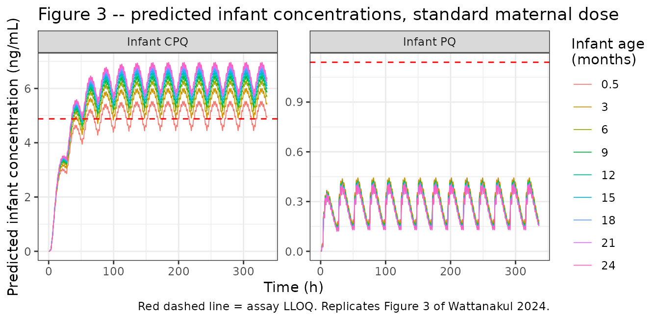
The paper reports that predicted median infant primaquine concentrations stay below the LLOQ in every scenario, and that roughly 70% of carboxyprimaquine concentrations are below theirs. The simulated profiles reproduce that: infant primaquine never reaches 1.14 ng/mL, while infant carboxyprimaquine crosses 4.88 ng/mL.
# Replicates Figures 5 and 6 of Wattanakul 2024: infant Cmax and AUC of
# primaquine plotted against infant age, one series per dosing scenario.
# Exposure over the same last-24-h-of-the-dosing-cycle window used for Table 3.
inf_exposure <- sim_inf |>
  filter(time >= last_dose + dose_ii - 24, time <= last_dose + dose_ii) |>
  group_by(scenario, AGE_INFANT, WT_INFANT) |>
  summarise(
    Cmax        = max(Cinfant)   * MW_PQ / 1000,
    AUC         = trapz(Cinfant, time) * MW_PQ / 1000,
    Cmax_mother = max(Cc)        * MW_PQ / 1000,
    AUC_mother  = trapz(Cc, time)      * MW_PQ / 1000,
    .groups = "drop"
  )

inf_exposure |>
  select(scenario, AGE_INFANT, Cmax, AUC) |>
  pivot_longer(c(Cmax, AUC), names_to = "metric", values_to = "value") |>
  mutate(metric = factor(metric, levels = c("Cmax", "AUC"),
                         labels = c("Figure 5: infant Cmax (ng/mL)",
                                    "Figure 6: infant AUC (ng*h/mL)"))) |>
  ggplot(aes(AGE_INFANT, value, colour = scenario)) +
  geom_line() + geom_point(size = 1) +
  facet_wrap(~metric, scales = "free_y") +
  labs(x = "Infant age (months)", y = NULL, colour = NULL,
       title = "Figures 5 and 6 -- infant primaquine exposure vs infant age",
       caption = "Replicates Figures 5 and 6 of Wattanakul 2024.") +
  theme_bw() +
  theme(legend.position = "bottom")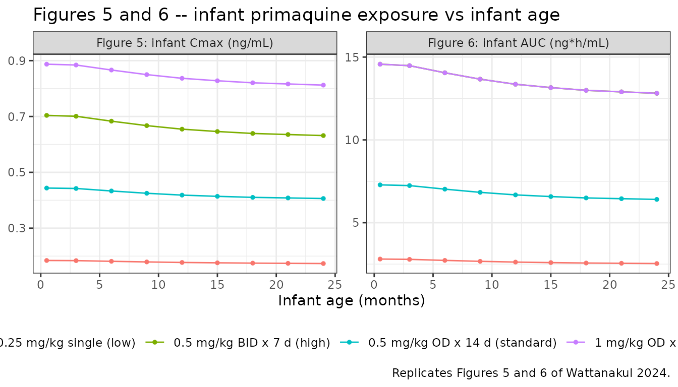
# The paper's headline safety claim: median predicted infant Cmax and AUC are
# more than 100-fold below the mother's in every dosing scenario.
ratios <- inf_exposure |>
  group_by(scenario) |>
  summarise(
    `Cmax fold-lower` = median(Cmax_mother / Cmax),
    `AUC fold-lower`  = median(AUC_mother  / AUC),
    .groups = "drop"
  )
knitr::kable(ratios, digits = 0,
caption = "Maternal:infant exposure ratio; the paper claims >100x.")| scenario | Cmax fold-lower | AUC fold-lower |
|---|---|---|
| 0.25 mg/kg single (low) | 320 | 200 |
| 0.5 mg/kg BID x 7 d (high) | 226 | 167 |
| 0.5 mg/kg OD x 14 d (standard) | 286 | 167 |
| 1 mg/kg OD x 7 d (high) | 286 | 167 |
# The paper additionally compares infant exposure with maternal exposure after
# a single low dose (0.25 mg base/kg), a level known not to cause significant
# haemolysis in G6PD-deficient individuals: Cmax 55.0 ng/mL, AUC 512 ng*h/mL.
c(max_infant_cmax_ng_mL = max(inf_exposure$Cmax),
  threshold_cmax_ng_mL  = 55.0,
  max_infant_auc        = max(inf_exposure$AUC),
  threshold_auc         = 512)
#> max_infant_cmax_ng_mL  threshold_cmax_ng_mL        max_infant_auc
#>             0.8872823            55.0000000            14.5701950
#>         threshold_auc
#>           512.0000000
stopifnot(max(inf_exposure$Cmax) < 55.0, max(inf_exposure$AUC) < 512)
Every simulated infant exposure is well below the maternal single-low-dose threshold, reproducing the paper’s safety conclusion.
Assumptions and deviations
Molecular weights are not in the paper. The models work in molar units (nmol, nmol/L) exactly as the source does. Converting to the ng/mL and ug*h/mL units of Table 2 and Table 3 requires the free-base molecular weights, which the paper does not state: 259.35 g/mol for primaquine and 274.32 g/mol for carboxyprimaquine were used here. These are chemical constants, used only in this vignette for unit presentation; no model parameter depends on them. Their correctness is supported by the agreement of all fourteen NCA parameters above – a wrong metabolite molecular weight would bias every carboxyprimaquine row by the same factor.
IIV on CL/F PQ: a 0.4 percentage-point table-vs-control-stream conflict. Table 2 reports 15.1 %CV, which implies
omega^2 = 0.0225; the control stream’s$OMEGA2 is 0.0214, which implies 14.71 %CV. All nine other random effects reproduce Table 2 to three significant figures under the paper’s own footnote-a formula, so the discrepancy is confined to this one term. The control-stream value is used, per the standing convention that an executable control stream beats a typeset table.Table 2’s
F_M (%)column header is wrong. The value 0.282 is a fraction, not a percentage. This is provable from the control stream’s$PKblock, which applies the logit transformLTF = LOG(TVFM/(1-TVFM)): that expression is only defined forTVFMin (0, 1), so 0.282 cannot be 28.2% read as 0.282%. The models encode it as a fraction.A typo in the control stream’s square wave. Both the Supplementary Information listing and the Zenodo deposit write
SQW2=(SQW-1)*(-1), referring to an undefined symbolSQW.SQW1is meant: Equation 8 defines the venous-to-milk wave as the complement of the milk-to-infant wave, and no otherSQWsymbol exists in the deck. Encoded assqwVenousToMilk = 1 - sqwMilkToInfant.The published PDF’s display equations cannot be trusted for the square wave. Extracting text from the article PDF drops the minus signs from Equations 5-8, so
S2 - S1reads asS2 S1– which would silently invert the feeding gate. The square-wave equations were transcribed from the control stream, not from the article text.A guard was added at the square wave’s switching instants. The published form
(sqrt(x^2) - x) / (2*sqrt(x^2))is 0/0 exactly whenx = 0, which happens twice per feeding cycle. The models evaluatesqrt(x^2 + 1e-12)instead. The offset is fifteen orders of magnitude below the wave’s amplitude, so it does not measurably soften the edge; it only keeps the expression finite. NONMEM avoided the issue by never landing exactly on the switching instant underADVAN13 TOL=6.IIV on the two partition coefficients and the two conversion factors is omitted, not written as
fixed(0). The authors estimated IIV on the conversion factors, found it at or below 10% with poor precision (%RSE 45 and 139), and fixed it to zero;$OMEGA9 and 10 are0 FIXand Table 2 reports “-” for all four. A zero-variance diagonal makes the OMEGA matrix singular and breaks the Cholesky sampler thatrxSolve()uses, so these terms carry no eta at all. The structural meaning – no between-subject variability on these parameters – is identical.Inter-occasion variability is expanded rather than expressed with
SAME. The source uses$OMEGA BLOCK(1)withSAMEon occasions 2-4, i.e. one shared variance across the four sampling occasions. nlmixr2 has noSAMEshortcut, so each occasion has its own eta with the variance fixed to the occasion-1 value, following the convention already used byJonsson_2011_ethambutolandAregbe_2012_alvespimycin.The conversion factor CF_PQ is 0.898, not the 0.902 quoted in the Results narrative. The 0.902 figure belongs to the earlier venous-plus-capillary model, fitted before the breast-milk data were introduced;
$THETA11 of the final deck and Table 2 both give 0.898.The maternal model does not drain the milk compartments. This is a structural inference, not a statement in the paper: the paper presents a single 17-compartment control stream and does not print the reduced maternal deck separately. It is settled empirically – Table 3’s milk:plasma AUC ratio of 0.376 (0.375-0.377) is reproduced exactly only without the drain, and gives about 0.28 with it (shown above). The distinction is why this paper contributes two model files.
The virtual cohort is not the study cohort. Individual data are not public. Maternal weights are drawn uniformly across the published range (35-81 kg, Table 1) rather than from the true distribution, and infant weight is held at the cohort median of 6.8 kg for the maternal simulations. Infant weight-for-age pairs in the dosing-scenario sweep are read off the WHO standard growth curves the paper cites, at the median z-score.
NCA comparisons are typical-value or small-cohort medians against 21-subject medians. The simulated cohort is 50 virtual mothers and the Table 3 replication is a single typical-value subject; the published values are medians over 21 women. Agreement to within a few percent should be read as confirming the structure and scaling, not as a formal statistical comparison. No parameter was tuned.
Infant predictions are extrapolation. No infant pharmacokinetic parameter was estimable: every infant capillary primaquine concentration except one (2.59 ng/mL) was below the LLOQ, and 67.5% of infant carboxyprimaquine concentrations were below theirs. The infant layer’s structure, allometric scaling, fixed absorption, and MAO-A maturation are assumptions carried from the mother and from the literature, evaluated only by overlaying a prediction interval on sparse below-LLOQ data (Figure 3).