Rocuronium and sugammadex in children (Grzeskowiak 2023)
Source:vignettes/articles/Grzeskowiak_2023_sugammadex_rocuronium.Rmd
Grzeskowiak_2023_sugammadex_rocuronium.RmdModel and source
- Citation: Grzeskowiak M, Bienert A, Wiczling P, Malec M, Grzelak J, Jarosz K, Ber J, Ksiazkiewicz M, Rosada-Kurasinska J, Grzeskowiak E, Bartkowska-Sniatkowska A. Population Pharmacokinetic-Pharmacodynamic Modeling and Probability of Target Attainment Analysis of Rocuronium and Sugammadex in Children Undergoing Surgery. Eur J Drug Metab Pharmacokinet. 2023;48:101-114. doi:10.1007/s13318-022-00809-1. Parameter values from Table S1 and the NONMEM control stream (S2) of Supplementary Material 2.
- Description: Bayesian population PK-PD model of rocuronium-induced neuromuscular blockade and its reversal by sugammadex in ASA I-II children aged 2.5-17 years (Grzeskowiak 2023). The structural model of Kleijn 2011 was refitted with informative priors: two-compartment PK for free rocuronium, free sugammadex and the rocuronium-sugammadex complex (complex PK set equal to sugammadex), dynamic complexation in the central compartments (kd fixed at 0.0559 uM, dissociation rate k2 estimated), a rocuronium effect compartment (ke0) driving a sigmoid Emax model of the train-of-four (TOF) ratio with E0 = Emax = 100 fixed, and a sugammadex-driven second-order elimination of rocuronium from the effect compartment (ks). Body weight is the only covariate: allometric exponents 1 on volumes, 0.75 on clearances and inter-compartmental clearances, and -0.25 on ke0 and ks, standardised to 70 kg. Posterior-mean parameter values; doses in umol, concentrations in uM, time in min.
- Article: https://doi.org/10.1007/s13318-022-00809-1
Grzeskowiak et al. refitted the Kleijn 2011 rocuronium-sugammadex
pharmacokinetic-pharmacodynamic model (available in this package as
Kleijn_2011_sugammadex_rocuronium) to paediatric data by
full Bayesian estimation, using the Kleijn 2011 estimates as informative
priors, and then used the posterior model to derive
probability-of-target-attainment (PTA) sugammadex doses. The model file
carries the posterior-mean parameters (Table S1 of Supplementary
Material 2) and the structural equations of the deposited NONMEM control
stream (S2).
Population
Thirty children aged 2.5-17 years (median 8.5) weighing 14-85 kg
(median 36.5 kg), 22 boys and 8 girls, ASA physical status I (n = 19) or
II (n = 11), undergoing surgery under propofol total intravenous
anaesthesia in Poznan, Poland (Results 3.1). All received rocuronium 0.6
mg/kg with maintenance boluses of half that dose when the TOF ratio
exceeded 40%, and sugammadex 0.5, 1.0 or 2.0 mg/kg at the end of surgery
(Methods 2.1). The analysis used 223 rocuronium and 130 sugammadex
plasma concentrations and 992 TOF-ratio measurements (Results 3.2). The
same information is available programmatically via
readModelDb("Grzeskowiak_2023_sugammadex_rocuronium")$population.
Source trace
Every ini() value carries an in-file comment pointing at
its source. The table consolidates them.
| Equation / parameter | Value | Source location |
|---|---|---|
| Sugammadex CL (CLS1), 70 kg | 0.093 L/min | Table S1A, posterior thetaP |
| Sugammadex V1 (VS1), 70 kg | 4.31 L | Table S1A, posterior thetaP |
| Sugammadex Q (CLS2), 70 kg | 0.206 L/min | Table S1A, posterior thetaP |
| Sugammadex V2 (VS2), 70 kg | 6.49 L | Table S1A, posterior thetaP |
| Rocuronium CL (CLR1), 70 kg | 0.278 L/min | Table S1A, posterior thetaP |
| Rocuronium V1 (VR1), 70 kg | 5.00 L | Table S1A, posterior thetaP |
| Rocuronium Q (CLR2), 70 kg | 0.284 L/min | Table S1A, posterior thetaP |
| Rocuronium V2 (VR2), 70 kg | 7.17 L | Table S1A, posterior thetaP |
Complex dissociation rate kOFF (k2) |
0.022 1/min | Table S1A, posterior thetaP |
| Equilibrium dissociation constant Kd (fixed) | 0.0559 uM | Methods 2.3; S2 $PK (KD = 0.0559) |
Association rate kON = kOFF / Kd (k1) |
derived | S2 $PK (KON = KOFF/KD) |
| Biophase equilibration kEO, 70 kg | 0.185 1/min | Table S1A, posterior thetaP |
| EC50R | 1.43 uM | Table S1A, posterior thetaP |
| Hill coefficient GAM | 6.96 | Table S1A, posterior thetaP |
| Sugammadex biophase elimination kS, 70 kg | 0.080 1/(uM min) | Table S1A, posterior thetaP |
| E0 and Emax (fixed) | 100 and 100 | Methods 2.3; S2 $ERROR
|
| IIV (13 diagonal elements) | 37.8-87.9% | Table S1B, posterior Omega |
| Proportional residual, rocuronium / sugammadex | 25.2% / 26.9% | Table S1C, posterior sigma |
| Additive residual, TOF ratio | 11.6 | Table S1C, posterior sigma |
| Allometric exponents 1 / 0.75 / -0.25 / 0, reference 70 kg | fixed | Methods 2.3 (Eqs. 1-2); S2 $PK (LNWT - 4.2485) |
| Two-compartment PK, complexation in central compartments | – | Methods 2.3; S2 $DES
|
| Biophase compartment with sugammadex-driven elimination | – | Methods 2.3; S2 $DES DADT(6) |
| Observed concentrations = free + complex | – | S2 $ERROR (CMT 1 and 2) |
| Molecular weights 527.8 (rocuronium) and 2002.2 (sugammadex) g/mol | – | Methods 2.3 |
Virtual cohort
The paper’s simulations (Section 2.4) use subjects of fixed body weight (5, 10, 20, 40 and 70 kg) dosed with rocuronium 0.6 mg/kg at time 0 and sugammadex 2, 5, 10 or 20 min later. Doses are converted from mg to umol with the molecular weights stated in Methods 2.3.
The between-subject random effects are drawn once in R (200 virtual
subjects) and passed to rxSolve() as fixed per-subject
values, so every dose arm and body weight is simulated with the same 200
subjects. That makes the PTA curves monotone in dose and makes the
cohort identical on every machine, whatever rxode2’s thread count.
mod <- readModelDb("Grzeskowiak_2023_sugammadex_rocuronium")
ui <- rxode2::rxode(mod)
#> ℹ parameter labels from comments will be replaced by 'label()'

MW_ROC <- 527.8 # g/mol, Methods 2.3
MW_SGX <- 2002.2 # g/mol, Methods 2.3
n_sub <- 200L

omega_sd <- sqrt(diag(ui$omega))
set.seed(20230101)
etas <- as.data.frame(
  matrix(rnorm(n_sub * length(omega_sd)), n_sub) %*% diag(omega_sd)
)
names(etas) <- names(omega_sd)
etas_zero <- etas[1, , drop = FALSE]
etas_zero[] <- 0

# One row per (arm, virtual subject). `arms` has columns WT (kg), tsgx (min
# after rocuronium) and sgx (sugammadex mg/kg; 0 = no sugammadex).
# Observation rows sit on the TOF endpoint `NMB`, a declared endpoint of the
# model; total concentrations (Cc, Cc_roc) are returned on every row. With
# three declared endpoints rxode2 rejects observation rows on an ODE state,
# and naming a declared endpoint adds no compartment slot (guarded below).
stopifnot(all(c("Cc", "Cc_roc", "NMB") %in% ui$predDf$cond))
build_sim <- function(arms, eta_df, obs_rel) {
  n <- nrow(eta_df)
  subj <- arms[rep(seq_len(nrow(arms)), each = n), , drop = FALSE]
  subj$id <- seq_len(nrow(subj))
  subj$subj <- rep(seq_len(n), times = nrow(arms))
  roc <- data.frame(
    id = subj$id, time = 0, amt = 0.6 * subj$WT / MW_ROC * 1000,
    cmt = "central_roc", evid = 1L
  )
  sg <- subj[subj$sgx > 0, , drop = FALSE]
  sgx <- data.frame(
    id = sg$id, time = sg$tsgx, amt = sg$sgx * sg$WT / MW_SGX * 1000,
    cmt = "central", evid = 1L
  )
  obs <- data.frame(
    id = rep(subj$id, each = length(obs_rel)),
    time = rep(subj$tsgx, each = length(obs_rel)) + rep(obs_rel, nrow(subj)),
    amt = 0, cmt = "NMB", evid = 0L
  )
  ev <- dplyr::bind_rows(roc, sgx, obs) |>
    dplyr::left_join(subj[, c("id", "WT")], by = "id") |>
    dplyr::arrange(id, time, dplyr::desc(evid))
  pars <- eta_df[subj$subj, , drop = FALSE]
  pars$id <- subj$id
  list(events = ev, params = pars, subj = subj)
}

run_sim <- function(x) {
  sim <- rxode2::rxSolve(
    ui, x$events,
    params = x$params, sigma = NA, useLinCmt = FALSE,
    returnType = "data.frame"
  )
  sim |>
    dplyr::select(id, time, Cc, Cc_roc, NMB, cl) |>
    dplyr::left_join(x$subj, by = "id") |>
    dplyr::mutate(trel = time - tsgx)
}

# Reversal time (Methods 2.4): time after the sugammadex dose after which the
# TOF ratio stays above 90%. Zero when the TOF ratio is already above 90% at
# the sugammadex dose; the end of the grid when it never recovers.
reversal_time <- function(sim) {
  sim |>
    dplyr::filter(trel >= 0) |>
    dplyr::group_by(id) |>
    dplyr::summarise(
      rt = {
        below <- trel[NMB <= 90]
        if (length(below) == 0) 0 else min(c(trel[trel > max(below)], max(trel)))
      },
      .groups = "drop"
    )
}
Simulation and replication of published results
Figure 4: 20 kg subject, sugammadex 20 min after rocuronium
arms_f4 <- data.frame(WT = 20, tsgx = 20, sgx = c(0, 0.5, 1, 2))
obs_f4 <- c(seq(-20, -0.5, by = 0.5), seq(0, 30, by = 0.25), seq(31, 600, by = 1))
sim_f4 <- run_sim(build_sim(arms_f4, etas, obs_f4)) |>
  dplyr::mutate(
    dose_lab = factor(paste(sgx, "mg/kg"), levels = paste(c(0, 0.5, 1, 2), "mg/kg")),
    Croc_ngmL = Cc_roc * MW_ROC,
    Csgx_ugmL = Cc * MW_SGX / 1000
  )

f4_sum <- sim_f4 |>
  dplyr::filter(time <= 180) |>
  tidyr::pivot_longer(c(Croc_ngmL, Csgx_ugmL, NMB), names_to = "panel") |>
  dplyr::group_by(panel, dose_lab, time) |>
  dplyr::summarise(
    mean = mean(value), lo = quantile(value, 0.05), hi = quantile(value, 0.95),
    .groups = "drop"
  ) |>
  dplyr::mutate(panel = factor(
    panel,
    levels = c("Croc_ngmL", "Csgx_ugmL", "NMB"),
    labels = c("Rocuronium, ng/mL", "Sugammadex, ug/mL", "TOF ratio, %")
  ))
ggplot(f4_sum, aes(time / 60, mean, colour = dose_lab, fill = dose_lab)) +
  geom_ribbon(aes(ymin = lo, ymax = hi), alpha = 0.15, colour = NA) +
  geom_line() +
  facet_wrap(~panel, ncol = 1, scales = "free_y") +
  labs(x = "Time, h", y = NULL, colour = "Sugammadex", fill = "Sugammadex") +
  theme_bw()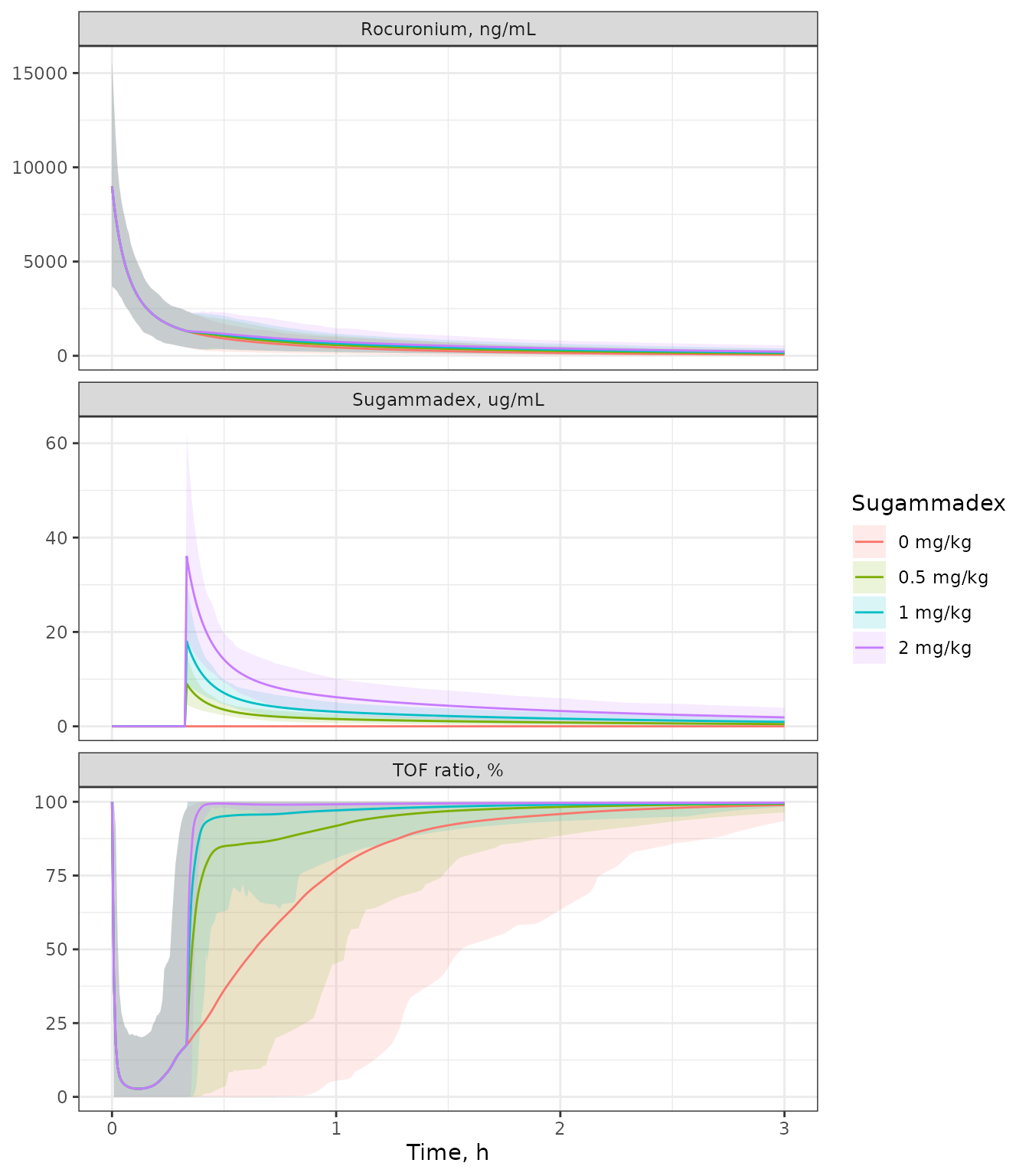
Replicates Figure 4 of Grzeskowiak 2023: mean (line) and 5th-95th percentiles (band) for a 20 kg subject given rocuronium 0.6 mg/kg and sugammadex 0, 0.5, 1 or 2 mg/kg 20 min later.
f4_prob <- sim_f4 |>
  dplyr::filter(time <= 180) |>
  dplyr::group_by(dose_lab, time) |>
  dplyr::summarise(p90 = 100 * mean(NMB > 90), .groups = "drop")
ggplot(f4_prob, aes(time / 60, p90, colour = dose_lab)) +
  geom_line() +
  labs(x = "Time, h", y = "TOF ratio > 90%, % subjects", colour = "Sugammadex") +
  theme_bw()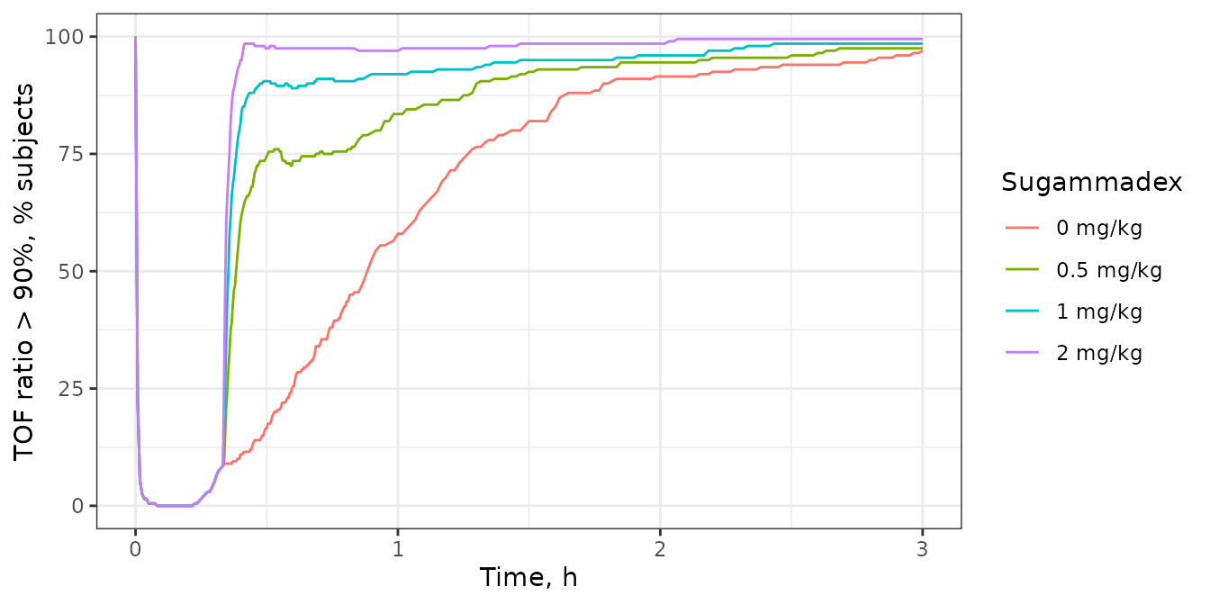
Replicates the bottom panel of Figure 4: percentage of 20 kg subjects with a TOF ratio above 90% over time.
# Read off the bottom panel of the published Figure 4 at 1 h.
f4_check <- f4_prob |>
  dplyr::filter(time == 60) |>
  dplyr::select(dose_lab, p90) |>
  dplyr::mutate(p90_pub = c(53, 80, 93, 99))
f4_check |>
  dplyr::rename(
    "Sugammadex" = dose_lab, "Simulated (%)" = p90,
    "Figure 4, digitised (%)" = p90_pub
  ) |>
knitr::kable(digits = 0, caption = "Subjects with TOF ratio > 90% at 1 h (40 min after sugammadex).")| Sugammadex | Simulated (%) | Figure 4, digitised (%) |
|---|---|---|
| 0 mg/kg | 58 | 53 |
| 0.5 mg/kg | 84 | 80 |
| 1 mg/kg | 92 | 93 |
| 2 mg/kg | 97 | 99 |
In the published bottom panel the curves for 0.5, 1 and 2 mg/kg rise to roughly 73%, 92% and 98% within minutes of the sugammadex dose, and the no-sugammadex curve passes 50% just before 1 h. The peak mean sugammadex concentration for 2 mg/kg is about 30 ug/mL.
sgx_peak <- sim_f4 |>
  dplyr::filter(sgx == 2, trel >= 0) |>
  dplyr::group_by(time) |>
  dplyr::summarise(m = mean(Csgx_ugmL), .groups = "drop")
stopifnot(
  # Typical C0 = 40 mg / 2002.2 g/mol / (4.31 L * 20/70) = 32 ug/mL; the
  # published mean peak is ~30 ug/mL. A wrong volume or MW moves this by >30%.
  abs(max(sgx_peak$m) / 30 - 1) < 0.3,
  # Reversal probability at 1 h within 15 percentage points of the digitised
  # figure (realised: within about 5). The published curves also carry
  # parameter uncertainty, which pulls them towards 50%.
  max(abs(f4_check$p90 - f4_check$p90_pub)) < 15
)
Table 1: reversal time
The paper simulated from the full posterior distribution (n = 4000 posterior draws, each with its own between-subject variability), so its spread includes parameter uncertainty. This model carries the posterior means only. The typical subject (all random effects zero) is therefore compared with the Table 1 median over the full 80-cell grid.
table1 <- tibble::tribble(
  ~WT, ~tsgx, ~sgx, ~mean_pub, ~median_pub, ~p05_pub, ~p95_pub,
  70, 2, 0.5, 65, 53, 15, 174, 70, 2, 1, 44, 30, 1, 145, 70, 2, 2, 15, 3, 0, 75, 70, 2, 4, 3, 1, 0, 7,
  70, 5, 0.5, 60, 48, 8, 170, 70, 5, 1, 37, 20, 1, 134, 70, 5, 2, 11, 3, 0, 63, 70, 5, 4, 3, 1, 0, 6,
  70, 10, 0.5, 51, 38, 3, 163, 70, 10, 1, 27, 7, 1, 118, 70, 10, 2, 7, 2, 0, 36, 70, 10, 4, 2, 1, 0, 5,
  70, 20, 0.5, 35, 9, 1, 145, 70, 20, 1, 15, 3, 0, 89, 70, 20, 2, 4, 1, 0, 9, 70, 20, 4, 1, 1, 0, 4,
  40, 2, 0.5, 57, 45, 12, 151, 40, 2, 1, 38, 25, 1, 126, 40, 2, 2, 13, 3, 0, 64, 40, 2, 4, 3, 1, 0, 6,
  40, 5, 0.5, 52, 41, 5, 147, 40, 5, 1, 31, 14, 1, 114, 40, 5, 2, 9, 2, 0, 52, 40, 5, 4, 2, 1, 0, 5,
  40, 10, 0.5, 43, 30, 2, 141, 40, 10, 1, 22, 5, 1, 102, 40, 10, 2, 6, 2, 0, 24, 40, 10, 4, 2, 1, 0, 4,
  40, 20, 0.5, 27, 6, 1, 123, 40, 20, 1, 11, 2, 0, 69, 40, 20, 2, 3, 1, 0, 6, 40, 20, 4, 1, 0, 0, 3,
  20, 2, 0.5, 48, 38, 9, 126, 20, 2, 1, 31, 20, 1, 105, 20, 2, 2, 11, 2, 0, 53, 20, 2, 4, 2, 1, 0, 5,
  20, 5, 0.5, 43, 32, 3, 122, 20, 5, 1, 24, 9, 1, 92, 20, 5, 2, 7, 2, 0, 40, 20, 5, 4, 2, 1, 0, 4,
  20, 10, 0.5, 34, 20, 1, 116, 20, 10, 1, 17, 3, 1, 80, 20, 10, 2, 5, 1, 0, 11, 20, 10, 4, 2, 1, 0, 3,
  20, 20, 0.5, 20, 3, 0, 97, 20, 20, 1, 9, 1, 0, 51, 20, 20, 2, 3, 1, 0, 4, 20, 20, 4, 1, 0, 0, 2,
  10, 2, 0.5, 40, 31, 7, 106, 10, 2, 1, 26, 16, 1, 86, 10, 2, 2, 9, 2, 0, 44, 10, 2, 4, 2, 1, 0, 4,
  10, 5, 0.5, 35, 26, 2, 102, 10, 5, 1, 19, 6, 1, 77, 10, 5, 2, 6, 1, 0, 31, 10, 5, 4, 2, 1, 0, 3,
  10, 10, 0.5, 26, 12, 1, 94, 10, 10, 1, 13, 2, 0, 64, 10, 10, 2, 4, 1, 0, 8, 10, 10, 4, 1, 0, 0, 3,
  10, 20, 0.5, 15, 2, 0, 77, 10, 20, 1, 6, 1, 0, 36, 10, 20, 2, 2, 0, 0, 3, 10, 20, 4, 1, 0, 0, 2,
  5, 2, 0.5, 33, 26, 4, 88, 5, 2, 1, 21, 12, 1, 71, 5, 2, 2, 7, 1, 0, 35, 5, 2, 4, 2, 1, 0, 3,
  5, 5, 0.5, 28, 20, 1, 84, 5, 5, 1, 15, 4, 0, 64, 5, 5, 2, 5, 1, 0, 22, 5, 5, 4, 2, 0, 0, 3,
  5, 10, 0.5, 20, 5, 1, 76, 5, 10, 1, 9, 2, 0, 51, 5, 10, 2, 3, 1, 0, 5, 5, 10, 4, 1, 0, 0, 2,
  5, 20, 0.5, 10, 1, 0, 59, 5, 20, 1, 4, 1, 0, 23, 5, 20, 2, 2, 0, 0, 2, 5, 20, 4, 1, 0, 0, 1
)

obs_rt <- c(seq(0, 10, by = 0.1), seq(10.5, 30, by = 0.5), seq(31, 240, by = 1))
x_typ <- build_sim(as.data.frame(table1[, c("WT", "tsgx", "sgx")]), etas_zero, obs_rt)
rt_typ <- reversal_time(run_sim(x_typ)) |>
  dplyr::left_join(x_typ$subj, by = "id") |>
  dplyr::select(WT, tsgx, sgx, rt_typical = rt) |>
  dplyr::left_join(table1, by = c("WT", "tsgx", "sgx"))

rt_typ |>
  dplyr::filter(sgx %in% c(0.5, 2)) |>
  dplyr::select(WT, tsgx, sgx, rt_typical, median_pub) |>
  dplyr::rename(
    "BW (kg)" = WT, "T_SGX (min)" = tsgx, "SGX (mg/kg)" = sgx,
    "Typical subject (min)" = rt_typical, "Table 1 median (min)" = median_pub
  ) |>
knitr::kable(digits = 1, caption = "Typical-subject reversal time against the Table 1 median (0.5 and 2 mg/kg rows shown).")| BW (kg) | T_SGX (min) | SGX (mg/kg) | Typical subject (min) | Table 1 median (min) |
|---|---|---|---|---|
| 70 | 2 | 0.5 | 54.0 | 53 |
| 70 | 2 | 2.0 | 3.2 | 3 |
| 70 | 5 | 0.5 | 50.0 | 48 |
| 70 | 5 | 2.0 | 2.7 | 3 |
| 70 | 10 | 0.5 | 41.0 | 38 |
| 70 | 10 | 2.0 | 2.0 | 2 |
| 70 | 20 | 0.5 | 7.1 | 9 |
| 70 | 20 | 2.0 | 1.2 | 1 |
| 40 | 2 | 0.5 | 46.0 | 45 |
| 40 | 2 | 2.0 | 2.7 | 3 |
| 40 | 5 | 0.5 | 42.0 | 41 |
| 40 | 5 | 2.0 | 2.3 | 2 |
| 40 | 10 | 0.5 | 34.0 | 30 |
| 40 | 10 | 2.0 | 1.6 | 2 |
| 40 | 20 | 0.5 | 4.7 | 6 |
| 40 | 20 | 2.0 | 1.0 | 1 |
| 20 | 2 | 0.5 | 39.0 | 38 |
| 20 | 2 | 2.0 | 2.3 | 2 |
| 20 | 5 | 0.5 | 34.0 | 32 |
| 20 | 5 | 2.0 | 1.8 | 2 |
| 20 | 10 | 0.5 | 24.0 | 20 |
| 20 | 10 | 2.0 | 1.2 | 1 |
| 20 | 20 | 0.5 | 2.9 | 3 |
| 20 | 20 | 2.0 | 0.7 | 1 |
| 10 | 2 | 0.5 | 32.0 | 31 |
| 10 | 2 | 2.0 | 1.8 | 2 |
| 10 | 5 | 0.5 | 27.5 | 26 |
| 10 | 5 | 2.0 | 1.4 | 1 |
| 10 | 10 | 0.5 | 8.1 | 12 |
| 10 | 10 | 2.0 | 0.9 | 1 |
| 10 | 20 | 0.5 | 1.8 | 2 |
| 10 | 20 | 2.0 | 0.5 | 0 |
| 5 | 2 | 0.5 | 26.5 | 26 |
| 5 | 2 | 2.0 | 1.5 | 1 |
| 5 | 5 | 0.5 | 21.5 | 20 |
| 5 | 5 | 2.0 | 1.1 | 1 |
| 5 | 10 | 0.5 | 4.0 | 5 |
| 5 | 10 | 2.0 | 0.7 | 1 |
| 5 | 20 | 0.5 | 1.2 | 1 |
| 5 | 20 | 2.0 | 0.3 | 0 |
big <- rt_typ |> dplyr::filter(median_pub >= 5)
small <- rt_typ |> dplyr::filter(median_pub < 5)
summary(abs(big$rt_typical / big$median_pub - 1))
#>    Min. 1st Qu.  Median    Mean 3rd Qu.    Max.
#> 0.01887 0.04018 0.10000 0.10742 0.12976 0.32500
stopifnot(
  nrow(big) >= 20L,
  # Where the published median is at least 5 min, the typical subject's
  # relative deviation from it is small at the median and bounded at the
  # 90th percentile. Wrong clearance, EC50 or ks values shift these long
  # reversal times by far more.
  median(abs(big$rt_typical / big$median_pub - 1)) < 0.15,
  quantile(abs(big$rt_typical / big$median_pub - 1), 0.9) < 0.35,
  # Where the published median is under 5 min (integer-rounded) the typical
  # subject reverses within 3 min of it.
  quantile(abs(small$rt_typical - small$median_pub), 0.9) < 3
)
The spread is checked on a subset of the grid (5 kg and 70 kg, sugammadex 2 or 20 min after rocuronium), with 200 virtual subjects per cell.
arms_t1 <- expand.grid(WT = c(70, 5), tsgx = c(2, 20), sgx = c(0.5, 1, 2, 4))
x_t1 <- build_sim(arms_t1, etas, obs_rt)
rt_t1 <- reversal_time(run_sim(x_t1)) |>
  dplyr::left_join(x_t1$subj, by = "id") |>
  dplyr::group_by(WT, tsgx, sgx) |>
  dplyr::summarise(
    mean_sim = mean(rt), median_sim = median(rt),
    p05_sim = quantile(rt, 0.05), p95_sim = quantile(rt, 0.95),
    .groups = "drop"
  ) |>
  dplyr::left_join(table1, by = c("WT", "tsgx", "sgx")) |>
  dplyr::arrange(dplyr::desc(WT), tsgx, sgx)

rt_t1 |>
  dplyr::mutate(
    Simulated = sprintf("%.0f, %.1f [%.1f-%.0f]", mean_sim, median_sim, p05_sim, p95_sim),
    Published = sprintf("%g, %g [%g-%g]", mean_pub, median_pub, p05_pub, p95_pub)
  ) |>
  dplyr::select(WT, tsgx, sgx, Simulated, Published) |>
  dplyr::rename("BW (kg)" = WT, "T_SGX (min)" = tsgx, "SGX (mg/kg)" = sgx) |>
knitr::kable(caption = "Reversal time, mean, median [5th-95th percentile], minutes: simulation against Table 1.")| BW (kg) | T_SGX (min) | SGX (mg/kg) | Simulated | Published |
|---|---|---|---|---|
| 70 | 2 | 0.5 | 63, 52.5 [8.3-182] | 65, 53 [15-174] |
| 70 | 2 | 1.0 | 42, 27.5 [0.6-184] | 44, 30 [1-145] |
| 70 | 2 | 2.0 | 17, 3.1 [0.2-72] | 15, 3 [0-75] |
| 70 | 2 | 4.0 | 4, 0.8 [0.1-6] | 3, 1 [0-7] |
| 70 | 20 | 0.5 | 35, 9.5 [0.8-162] | 35, 9 [1-145] |
| 70 | 20 | 1.0 | 18, 2.7 [0.4-122] | 15, 3 [0-89] |
| 70 | 20 | 2.0 | 7, 1.2 [0.2-9] | 4, 1 [0-9] |
| 70 | 20 | 4.0 | 3, 0.6 [0.1-3] | 1, 1 [0-4] |
| 5 | 2 | 0.5 | 33, 25.2 [3.6-92] | 33, 26 [4-88] |
| 5 | 2 | 1.0 | 20, 10.2 [0.5-92] | 21, 12 [1-71] |
| 5 | 2 | 2.0 | 9, 1.4 [0.2-35] | 7, 1 [0-35] |
| 5 | 2 | 4.0 | 3, 0.5 [0.1-3] | 2, 1 [0-3] |
| 5 | 20 | 0.5 | 11, 1.2 [0.0-63] | 10, 1 [0-59] |
| 5 | 20 | 1.0 | 6, 0.6 [0.0-38] | 4, 1 [0-23] |
| 5 | 20 | 2.0 | 3, 0.3 [0.0-2] | 2, 0 [0-2] |
| 5 | 20 | 4.0 | 1, 0.2 [0.0-1] | 1, 0 [0-1] |
long <- rt_t1 |> dplyr::filter(median_pub >= 5)
stopifnot(
  nrow(long) == 5L,
  # Mean reversal time where it is long enough to be resolved: within 30% of
  # Table 1 (realised: within about 20%).
  all(abs(rt_t1$mean_sim[rt_t1$mean_pub >= 10] / rt_t1$mean_pub[rt_t1$mean_pub >= 10] - 1) < 0.3),
  median(abs(long$median_sim / long$median_pub - 1)) < 0.3
)
Table 2: sugammadex dose for 90% probability of target attainment
For each cell, the 200 virtual subjects are simulated over a grid of sugammadex doses, the fraction reversing within the target time is computed, and the dose at which that fraction first reaches 0.9 is interpolated.
pta_cells <- data.frame(WT = c(70, 70, 20, 5), tsgx = c(2, 20, 20, 20))
dose_grid <- seq(0.4, 6, by = 0.2)
obs_pta <- c(seq(0, 10, by = 0.25), seq(11, 120, by = 1))
table2 <- tibble::tribble(
  ~WT, ~tsgx, ~target, ~dose_pub,
  70, 2, 3, 4.8, 70, 20, 3, 3.2, 20, 20, 3, 1.9, 5, 20, 3, 1.1,
  70, 2, 5, 3.8, 70, 20, 5, 2.0, 20, 20, 5, 1.3, 5, 20, 5, 0.9
)

dose_at_pta <- function(dose, pta, p = 0.9) {
  i <- which(pta >= p)[1]
  if (is.na(i)) {
    return(NA_real_)
  }
  if (i == 1) {
    return(dose[1])
  }
  dose[i - 1] + (p - pta[i - 1]) / (pta[i] - pta[i - 1]) * (dose[i] - dose[i - 1])
}

pta_res <- lapply(seq_len(nrow(pta_cells)), function(k) {
  arms <- data.frame(WT = pta_cells$WT[k], tsgx = pta_cells$tsgx[k], sgx = dose_grid)
  x <- build_sim(arms, etas, obs_pta)
  rt <- reversal_time(run_sim(x)) |> dplyr::left_join(x$subj, by = "id")
  rt |>
    dplyr::group_by(WT, tsgx, sgx) |>
    dplyr::summarise(pta3 = mean(rt < 3), pta5 = mean(rt < 5), .groups = "drop")
}) |>
  dplyr::bind_rows()

pta_dose <- pta_res |>
  dplyr::group_by(WT, tsgx) |>
  dplyr::summarise(
  `3` = dose_at_pta(sgx, pta3), `5` = dose_at_pta(sgx, pta5), .groups = "drop"
  ) |>
  tidyr::pivot_longer(c(`3`, `5`), names_to = "target", values_to = "dose_sim") |>
  dplyr::mutate(target = as.numeric(target)) |>
  dplyr::left_join(table2, by = c("WT", "tsgx", "target"))

pta_dose |>
  dplyr::rename(
    "BW (kg)" = WT, "T_SGX (min)" = tsgx, "Target reversal (min)" = target,
    "Simulated dose (mg/kg)" = dose_sim, "Table 2 dose (mg/kg)" = dose_pub
  ) |>
knitr::kable(digits = 2, caption = "Sugammadex dose giving PTA >= 0.9 after rocuronium 0.6 mg/kg: simulation against Table 2.")| BW (kg) | T_SGX (min) | Target reversal (min) | Simulated dose (mg/kg) | Table 2 dose (mg/kg) |
|---|---|---|---|---|
| 5 | 20 | 3 | 1.32 | 1.1 |
| 5 | 20 | 5 | 0.93 | 0.9 |
| 20 | 20 | 3 | 2.13 | 1.9 |
| 20 | 20 | 5 | 1.40 | 1.3 |
| 70 | 2 | 3 | 4.80 | 4.8 |
| 70 | 2 | 5 | 3.80 | 3.8 |
| 70 | 20 | 3 | 3.40 | 3.2 |
| 70 | 20 | 5 | 2.20 | 2.0 |
ggplot(pta_res, aes(sgx, pta3, colour = paste0(WT, " kg, ", tsgx, " min"))) +
  geom_line() +
  geom_hline(yintercept = 0.9, linetype = 2) +
  labs(x = "Sugammadex dose, mg/kg", y = "PTA (reversal < 3 min)", colour = "BW, T_SGX") +
  theme_bw()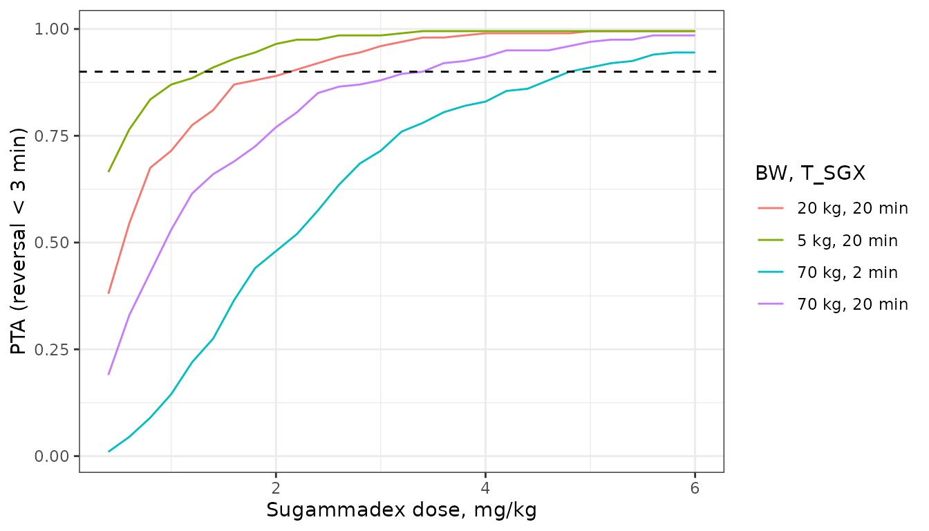
PTA curves in the style of Figure 5: probability of reversal (TOF ratio > 90%) within 3 min of the sugammadex dose.
stopifnot(
  !anyNA(pta_dose$dose_sim),
  # The PTA dose is a 90th-percentile statistic, so it is the part of the
  # analysis most sensitive to the missing parameter uncertainty; 30% still
  # catches a wrong ks, EC50 or volume (realised: within about 20%).
  median(abs(pta_dose$dose_sim / pta_dose$dose_pub - 1)) < 0.2,
  all(abs(pta_dose$dose_sim / pta_dose$dose_pub - 1) < 0.35)
)
PKNCA validation
The paper reports no non-compartmental results. The model does, however, fix one exact identity: free and complexed sugammadex share the same volumes and clearances and complexation only moves sugammadex between the two forms, so the measured (total) sugammadex follows linear two-compartment kinetics and its AUC from the dose to infinity equals dose / CL for every subject. PKNCA on the first 50 virtual subjects of each sugammadex arm of the Figure 4 simulation, sampled at a nominal 24-point schedule over 10 h, recovers that.
n_nca <- 50L
nca_times <- c(
  0, 0.5, 1, 2, 3, 5, 7.5, 10, 15, 20, 30, 45, 60, 90, 120, 150, 180,
  240, 300, 360, 420, 480, 540, 600
)
nca_conc <- sim_f4 |>
  dplyr::filter(sgx > 0, subj <= n_nca, trel %in% nca_times, !is.na(Cc)) |>
  dplyr::transmute(id, time = trel, Cc, treatment = dose_lab)
nca_dose <- sim_f4 |>
  dplyr::filter(sgx > 0, subj <= n_nca) |>
  dplyr::distinct(id, sgx, WT, dose_lab) |>
  dplyr::transmute(id, time = 0, amt = sgx * WT / MW_SGX * 1000, treatment = dose_lab)

conc_obj <- PKNCA::PKNCAconc(nca_conc, Cc ~ time | treatment + id)
dose_obj <- PKNCA::PKNCAdose(nca_dose, amt ~ time | treatment + id)
intervals <- data.frame(
  start = 0, end = Inf, cmax = TRUE, tmax = TRUE,
  aucinf.obs = TRUE, half.life = TRUE
)
nca_res <- PKNCA::pk.nca(PKNCA::PKNCAdata(conc_obj, dose_obj, intervals = intervals))
summary(nca_res)
#>  start end treatment  N        cmax                 tmax   half.life aucinf.obs
#>      0 Inf 0.5 mg/kg 50 4.11 [37.3] 0.000 [0.000, 0.000] 82.3 [36.2] 140 [33.6]
#>      0 Inf   1 mg/kg 50 8.23 [37.3] 0.000 [0.000, 0.000] 82.3 [36.2] 280 [33.6]
#>      0 Inf   2 mg/kg 50 16.5 [37.3] 0.000 [0.000, 0.000] 82.3 [36.2] 560 [33.6]
#>
#> Caption: cmax, aucinf.obs: geometric mean and geometric coefficient of variation; tmax: median and range; half.life: arithmetic mean and standard deviation; N: number of subjects
auc_check <- as.data.frame(nca_res$result) |>
  dplyr::filter(PPTESTCD == "aucinf.obs") |>
  dplyr::left_join(nca_dose, by = c("treatment", "id")) |>
  dplyr::left_join(
    sim_f4 |> dplyr::distinct(id, cl),
    by = "id"
  ) |>
  dplyr::mutate(pct_diff = 100 * (PPORRES / (amt / cl) - 1))
summary(auc_check$pct_diff)
#>    Min. 1st Qu.  Median    Mean 3rd Qu.    Max.
#> 0.01287 0.17419 0.25890 0.25582 0.31902 0.51007
stopifnot(
  nrow(auc_check) == 3L * n_nca,
  # Same parameters on both sides; the residual difference is the trapezoid
  # and log-linear extrapolation error of the NCA.
  abs(median(auc_check$pct_diff)) < 2,
  quantile(abs(auc_check$pct_diff), 0.9) < 5
)
Assumptions and deviations
- Posterior means, not the posterior distribution. The paper’s simulations draw from 4000 posterior samples, so their spread includes parameter uncertainty; this model holds the posterior-mean values from Table S1. Typical-subject reversal times match the Table 1 medians, while the simulated 95th percentiles of reversal time and the PTA doses are slightly smaller than published, as expected when parameter uncertainty is left out.
-
Between-subject variance scale. Table S1 reports
the variability as a percentage; the prior Omega0 of “30%” corresponds
to the control stream’s
$OMEGAPdiagonal of 0.09, so the percentage is 100 * sqrt(omega^2) and each variance is (percentage / 100)^2. -
Unreported covariances. The control stream
estimates two full
$OMEGAblocks (8 PK and 5 PD random effects), but only the diagonal elements are reported. The model uses a diagonal matrix. -
TOF residual error. Table S1 gives the posterior
TOF residual as 11.6. The table’s prior entry (2.70) is the
$SIGMAPvalue, which NONMEM reads as a variance, so 11.6 could in principle be a variance (SD 3.4). It is encoded as a standard deviation: the proportional residuals in the same table are standard deviations, and the scatter of observed against individual-predicted TOF ratio in the paper’s goodness-of-fit plot (Supplementary Material 2, Fig. 2S-B) is far wider than an SD of 3.4. The residual does not enter the simulations above. -
Kd units. Methods 2.3 prints the fixed dissociation
constant as 0.0559 mM; the control stream applies 0.0559 on the
micromolar scale of the
$DESblock, matching Kleijn 2011. The model uses 0.0559 uM. -
Complexation flux as coded. The deposited
$DESscales the complexation flux by the rocuronium central volume in the rocuronium equation and by the sugammadex central volume in the sugammadex and complex equations, so rocuronium amount is not conserved exactly through complexation. The model reproduces the deposited equations term for term; the publishedKleijn_2011_sugammadex_rocuroniummodel uses the sugammadex volume in all three. - Differences from Kleijn 2011. This refit has no age, creatinine clearance, race or sevoflurane covariates, scales sugammadex clearance allometrically, fixes E0 at 100 without variability, and puts random effects on all 13 structural parameters.
- Reversal time on a grid. Reversal time is read off a 0.1-min grid for the first 10 min after sugammadex (0.25 min for the PTA grid) and a coarser grid afterwards, up to 240 min (120 min for the PTA grid).
- Rocuronium maintenance doses. The study gave maintenance boluses when the TOF ratio exceeded 40%; like the paper’s own simulations, the simulations here give a single 0.6 mg/kg rocuronium dose.