Cefepime, meropenem and piperacillin-tazobactam in cystic fibrosis (Rolsma 2025)

Model and source

Rolsma et al. fitted four independent one-compartment population PK models – one each for cefepime, meropenem, piperacillin and tazobactam – to opportunistic plasma samples from children and adults with cystic fibrosis (CF). Because the four models were estimated separately, with different covariates and different interoccasion-variability structures, they are packaged as four model files that share this one vignette.

cefepime     <- readModelDb("Rolsma_2025_cefepime")
meropenem    <- readModelDb("Rolsma_2025_meropenem")
piperacillin <- readModelDb("Rolsma_2025_piperacillin")
tazobactam   <- readModelDb("Rolsma_2025_tazobactam")

• Citation: Rolsma SL, Sokolow A, Patel PC, Sokolow K, Jimenez-Truque N, Fissell WH, Ryan V, Kirkpatrick CM, Nation RL, Gu K, Teresi M, Fishbane N, Kontos M, An G, Winokur P, Landersdorfer CB, Creech CB (2025). Population Pharmacokinetic Modeling of Cefepime, Meropenem, and Piperacillin-Tazobactam in Patients With Cystic Fibrosis. The Journal of Infectious Diseases 231(2):e364-e374. doi:10.1093/infdis/jiae451. Final parameter estimates from Supplemental Table 6A.
• Article: https://doi.org/10.1093/infdis/jiae451
• Supplement (parameter estimates, Supplemental Table 6): https://doi.org/10.1093/infdis/jiae451 (open-access supplementary data, jiae451_supplementary_data.zip)

The main article reports no parameter values at all – it states only that “the estimates of the PK parameters from the final model are provided in Supplementary Table 6”. Every structural parameter, covariate reference value, variance and residual-error term in these four model files therefore comes from the supplement, not from the article body.

#> ℹ parameter labels from comments will be replaced by 'label()'

m – One-compartment population PK model with linear elimination for intravenously infused cefepime in children and adults with cystic fibrosis (Rolsma 2025; 82 participants / 96 enrollments, 368 plasma concentrations, ages 3 to 54 years). Total clearance is the sum of a renal arm proportional to lean-body-weight-based creatinine clearance (2.84 L/h at CLCR,LBW = 77 mL/min) and a constant non-renal arm (0.928 L/h), giving 3.77 L/h at the cohort reference. The central volume of distribution scales linearly with fat-free mass (9.95 L at 33 kg; the source reports fat-free mass as ‘lean body weight’ by the Janmahasatian formula). Correlated interindividual variability on renal clearance and volume (correlation 0.67) with a combined proportional plus additive residual error. CFTR modulator use, CFTR genotype and CF-related complications were screened and had no substantial effect.

#> ℹ parameter labels from comments will be replaced by 'label()'

m – One-compartment population PK model with linear elimination for intravenously infused meropenem in adolescents and adults with cystic fibrosis (Rolsma 2025; 42 participants / 50 enrollments, 192 plasma concentrations, ages 13 to 65 years). Total clearance is the sum of a renal arm proportional to lean-body-weight-based creatinine clearance (6.44 L/h at CLCR,LBW = 90 mL/min) and a non-renal arm scaling allometrically with total body weight (4.01 L/h at 61 kg, exponent 0.75), giving 10.5 L/h at the cohort reference. The central volume is 17.5 L with no covariate. Independent interindividual variability on renal clearance and volume, combined proportional plus additive residual error. CFTR modulator use, CFTR genotype and CF-related complications were screened and had no substantial effect.

#> ℹ parameter labels from comments will be replaced by 'label()'
#> Warning: some etas defaulted to non-mu referenced, possible parsing error: etaiov_cl_1, etaiov_cl_2, etaiov_cl_3
#> as a work-around try putting the mu-referenced expression on a simple line

m – One-compartment population PK model with linear elimination for the piperacillin component of intravenously infused piperacillin-tazobactam in children and adults with cystic fibrosis (Rolsma 2025; 31 participants / 34 enrollments, 107 plasma concentrations shared with tazobactam, ages 5 to 54 years). No covariate reached significance: clearance is 8.81 L/h and the central volume 12.2 L for every subject. Strongly correlated interindividual variability on clearance and volume (correlation 0.82) plus interoccasion variability on clearance across 3 occasions, with a combined proportional plus additive residual error. The companion tazobactam model is Rolsma_2025_tazobactam.

#> ℹ parameter labels from comments will be replaced by 'label()'
#> Warning: some etas defaulted to non-mu referenced, possible parsing error: etaiov_vc_1, etaiov_vc_2, etaiov_vc_3
#> as a work-around try putting the mu-referenced expression on a simple line

m – One-compartment population PK model with linear elimination for the tazobactam component of intravenously infused piperacillin-tazobactam in children and adults with cystic fibrosis (Rolsma 2025; 31 participants / 34 enrollments, 107 plasma concentrations shared with piperacillin, ages 5 to 54 years). No covariate reached significance: clearance is 7.67 L/h and the central volume 13.0 L for every subject. Strongly correlated interindividual variability on clearance and volume (correlation 0.93) plus interoccasion variability on the volume across 3 occasions, with a combined proportional plus additive residual error. The companion piperacillin model is Rolsma_2025_piperacillin.

Population

82 participants received cefepime, 42 meropenem and 31 piperacillin-tazobactam, out of 133 unique participants and 180 enrollments (participants could enrol more than once). 667 plasma samples were analysed: 368 cefepime, 192 meropenem and 107 piperacillin/tazobactam.

Baseline characteristics by antibiotic group (Rolsma 2025 Supplemental Tables 2 and 3). Ranges are minimum to maximum.

Characteristic	Cefepime	Meropenem	Piperacillin-tazobactam
Participants (enrollments)	82 (96)	42 (50)	31 (34)
Plasma samples	368	192	107
Age, median (range), y	15.0 (3-54)	29.5 (13-65)	22.0 (5-54)
Total body weight, median, kg	46.86 (13.6-102.5)	61.30 (36.3-137.0)	54.05 (17.6-93.3)
Lean body weight, median, kg	33.45 (11.1-69.5)	49.15 (26.7-63.5)	38.25 (13.6-59.3)
Body mass index, median, kg/m^2	19.15 (13.0-35.7)	20.45 (14.8-50.3)	20.15 (15.4-33.1)
Female, %	54	48	53
White, %	97	98	91
Age < 17 y, %	65	6	21
Any CFTR modulator use, %	35	48	35
At least one DF508 allele, %	95	96	97

All participants had confirmed CF and were admitted for a pulmonary exacerbation or for microbial eradication therapy at Vanderbilt University Medical Center or the University of Iowa Hospital between January 2018 and March 2020. Participants with prior solid-organ or hematologic transplantation were excluded.

Source trace

Every equation and every ini() value, with the exact location it came from. CLCR,LBW is creatinine clearance computed with the Cockcroft-Gault equation using lean body weight (subjects over 12 years) or the Schwartz bedside equation (subjects up to 12 years), in raw mL/min.

Source trace for the four Rolsma 2025 models. ‘Supplemental Table 6’ is in jiae451_supplementary_data.zip.

Model	Quantity	Value	Source
all	One-compartment, linear elimination, zero-order IV input	–	Results ‘PopPK Modeling’; Methods ‘PopPK Model Development’
all	Exponential IIV; combined additive + proportional residual error	–	Supplemental Methods ‘Population Pharmacokinetic Model Development’
cefepime	CL_R	2.84 L/h per 77 mL/min CLCR,LBW	Supplemental Table 6A
cefepime	CL_NR	0.928 L/h	Supplemental Table 6A
cefepime	CL total at reference	3.77 L/h	Supplemental Table 6A footnote a
cefepime	V	9.95 L per 33 kg LBW	Supplemental Table 6A
cefepime	IIV CL_R / V; correlation	22% / 22% CV; 0.67	Supplemental Table 6A
cefepime	Residual proportional / additive	33% / 0.241 mg/L	Supplemental Table 6A (CVCP, SDCP)
meropenem	CL_R	6.44 L/h per 90 mL/min CLCR,LBW	Supplemental Table 6B
meropenem	CL_NR (BMI < 45)	4.01 L/h per 61 kg^0.75 TBW	Supplemental Table 6B
meropenem	CL total at reference	10.5 L/h	Supplemental Table 6B footnote a
meropenem	V	17.5 L	Supplemental Table 6B
meropenem	IIV CL_R / V	21% / 14% CV (independent)	Supplemental Table 6B
meropenem	Residual proportional / additive	41% / 0.315 mg/L	Supplemental Table 6B
piperacillin	CL / V	8.81 L/h / 12.2 L	Supplemental Table 6C
piperacillin	IIV CL / V; correlation	56% / 85% CV; 0.82	Supplemental Table 6C
piperacillin	IOV on CL (3 occasions)	29% CV	Supplemental Table 6C caption + Results
piperacillin	Residual proportional / additive	47% / 0.872 mg/L	Supplemental Table 6C
tazobactam	CL / V	7.67 L/h / 13.0 L	Supplemental Table 6D
tazobactam	IIV CL / V; correlation	55% / 79% CV; 0.93	Supplemental Table 6D
tazobactam	IOV on V (3 occasions)	54% CV	Supplemental Table 6D caption + Results
tazobactam	Residual proportional / additive	43% / 0.548 mg/L	Supplemental Table 6D
PTA	Protein binding: cefepime / meropenem / piperacillin	20% / 2% / 30%	Methods, PTA paragraph
PTA	Published breakpoints	see Table 1	Table 1

Reading the covariate model out of the unit strings

Supplemental Table 6 does not print covariate equations. It encodes them in the Unit column, and the table’s own footnotes provide a mass-balance check that confirms the reading:

• Cefepime CL_R has unit “L/h per 77 mL/min CLCR,LBW”, i.e. CL_R = 2.84 x (CLCR / 77), and V has unit “L per 33 kg LBW”, i.e. V = 9.95 x (LBW / 33). Footnote a gives total CL = 3.77 L/h “for a CL_CR,LBW of 77 mL/min”, and 2.84 + 0.928 = 3.768, which rounds to 3.77.
• Meropenem CL_R has unit “L/h per 90 mL/min CLCR,LBW” and CL_NR has unit “L/h/61kg^0.75 TBW”, i.e. CL_NR = 4.01 x (TBW / 61)^0.75. Footnote a gives total CL = 10.5 L/h “for the typical CL_CR and TBW in the study population”, and 6.44 + 4.01 = 10.45, which rounds to 10.5.

Both reference values are also the cohort medians in Supplemental Table 3 (lean body weight 33.45 kg for cefepime, total body weight 61.30 kg for meropenem), which independently corroborates the reading. Neither table reports an exponent parameter for the two normalisations, so both are linear rather than power relationships; the only exponent in the four models is the 0.75 printed inside the meropenem CL_NR unit string, which has no row, estimate or standard error of its own and is therefore encoded as fixed.

Structural check: reproduce the published total clearances

The first gate is that the packaged models reproduce Supplemental Table 6’s footnoted total clearances at the reference covariate values.

typ <- function(mod, covs) {
  ev <- rxode2::et(amt = 1000, dur = 1, cmt = "central") |>
    rxode2::et(c(0, 1, 2), cmt = "central")
  d <- as.data.frame(ev)
  for (nm in names(covs)) d[[nm]] <- covs[[nm]]
  for (e in rxode2::rxode(mod)$iniDf$name[!is.na(rxode2::rxode(mod)$iniDf$neta1)]) d[[e]] <- 0
  rxode2::rxSolve(mod, d, omega = NA, sigma = NA, returnType = "data.frame")
}

cl_cefepime  <- unique(round(typ(cefepime,  list(CRCL = 77, FFM = 33))$cl, 3))
#> ℹ parameter labels from comments will be replaced by 'label()'
#> ℹ parameter labels from comments will be replaced by 'label()'
#> ℹ parameter labels from comments will be replaced by 'label()'
cl_meropenem <- unique(round(typ(meropenem, list(CRCL = 90, WT = 61))$cl, 3))
#> ℹ parameter labels from comments will be replaced by 'label()'
#> ℹ parameter labels from comments will be replaced by 'label()'
#> ℹ parameter labels from comments will be replaced by 'label()'

total_cl <- tibble::tibble(
  Model      = c("cefepime", "meropenem"),
  Reference  = c("CLCR,LBW = 77 mL/min, LBW = 33 kg", "CLCR,LBW = 90 mL/min, TBW = 61 kg"),
  Simulated  = c(cl_cefepime, cl_meropenem),
  Published  = c(3.77, 10.5),
  Source     = c("Suppl Table 6A footnote a", "Suppl Table 6B footnote a")
)
knitr::kable(total_cl, digits = 3,
             caption = "Total clearance at the reference covariate values (L/h). Both reproduce the published footnoted totals to rounding.")

Total clearance at the reference covariate values (L/h). Both reproduce the published footnoted totals to rounding.

Model	Reference	Simulated	Published	Source
cefepime	CLCR,LBW = 77 mL/min, LBW = 33 kg	3.768	3.77	Suppl Table 6A footnote a
meropenem	CLCR,LBW = 90 mL/min, TBW = 61 kg	10.450	10.50	Suppl Table 6B footnote a

Virtual cohorts

Covariate distributions are reconstructed from Supplemental Table 3. Two quantities the paper does not publish have to be assumed and are flagged in “Assumptions and deviations” below: the distribution of CLCR,LBW, and the lean-to-total weight relationship.

N_ARM <- 200  # participants per simulated arm

# Log-normal draw matched to a published arithmetic mean and SD, clipped to the
# published min-max range.
rln <- function(n, mean, sd, lo, hi) {
  s2 <- log(1 + (sd / mean)^2)
  x  <- rlnorm(n, log(mean) - s2 / 2, sqrt(s2))
  pmin(pmax(x, lo), hi)
}

# Cefepime: total body weight from Suppl Table 3; lean body weight derived from
# it with the cohort mean lean:total ratio (34.74 / 46.71 = 0.744).
cohort_cefepime <- tibble::tibble(
  id   = seq_len(N_ARM),
  WT   = rln(N_ARM, 46.71, 18.68, 13.6, 102.5),
  CRCL = rln(N_ARM, 77, 77 * 0.30, 20, 250)
) |>
  mutate(FFM = 0.744 * WT,
         # Published pediatric rule: 50 mg/kg per dose, maximum 2000 mg.
         dose_mg = pmin(50 * WT, 2000))

# Meropenem: total body weight from Suppl Table 3; volume takes no covariate.
cohort_meropenem <- tibble::tibble(
  id   = seq_len(N_ARM),
  WT   = rln(N_ARM, 62.21, 19.51, 36.3, 137.0),
  CRCL = rln(N_ARM, 90, 90 * 0.30, 25, 250)
)

# Piperacillin / tazobactam: NO covariates were retained, so the cohort needs no
# covariate reconstruction at all -- only the occasion indicator.
cohort_piperacillin <- tibble::tibble(id = seq_len(N_ARM), OCC = 1)

knitr::kable(
  tibble::tibble(
    Cohort = c("cefepime", "cefepime", "cefepime", "meropenem", "meropenem"),
    Covariate = c("WT (kg)", "FFM (kg)", "CLCR (mL/min)", "WT (kg)", "CLCR (mL/min)"),
    Median = c(median(cohort_cefepime$WT), median(cohort_cefepime$FFM),
               median(cohort_cefepime$CRCL), median(cohort_meropenem$WT),
               median(cohort_meropenem$CRCL)),
    `5th pct` = c(quantile(cohort_cefepime$WT, .05), quantile(cohort_cefepime$FFM, .05),
                  quantile(cohort_cefepime$CRCL, .05), quantile(cohort_meropenem$WT, .05),
                  quantile(cohort_meropenem$CRCL, .05)),
    `95th pct` = c(quantile(cohort_cefepime$WT, .95), quantile(cohort_cefepime$FFM, .95),
                   quantile(cohort_cefepime$CRCL, .95), quantile(cohort_meropenem$WT, .95),
                   quantile(cohort_meropenem$CRCL, .95))
  ), digits = 1, caption = "Simulated covariate distributions (200 participants per arm)."
)

Simulated covariate distributions (200 participants per arm).

Cohort	Covariate	Median	5th pct	95th pct
cefepime	WT (kg)	44.2	24.6	80.8
cefepime	FFM (kg)	32.9	18.3	60.1
cefepime	CLCR (mL/min)	74.0	46.8	124.8
meropenem	WT (kg)	59.2	36.4	96.9
meropenem	CLCR (mL/min)	87.4	52.4	142.9

Simulation and NCA validation

For a one-compartment model with zero-order input the NCA metrics have exact closed forms, so PKNCA run on a noise-free typical-value profile must return the ini() clearance and volume back. This is the strongest available check that the structural implementation, the covariate equations and the unit system are all correct: AUC(0-inf) = Dose / CL, Cmax = Dose / (CL x T_inf) x (1 - exp(-kel x T_inf)) and t1/2 = ln(2) x V / CL.

sim_typical <- function(mod, amt, dur, covs, label, tmax = 24) {
  ev <- rxode2::et(amt = amt, dur = dur, cmt = "central") |>
    rxode2::et(sort(unique(c(seq(0, tmax, by = 0.05), dur))), cmt = "central")
  d <- as.data.frame(ev)
  for (nm in names(covs)) d[[nm]] <- covs[[nm]]
  for (e in rxode2::rxode(mod)$iniDf$name[!is.na(rxode2::rxode(mod)$iniDf$neta1)]) d[[e]] <- 0
  s <- rxode2::rxSolve(mod, d, omega = NA, sigma = NA, returnType = "data.frame")
  s$treatment <- label
  s$id <- 1L
  s
}

typ_profiles <- bind_rows(
  sim_typical(cefepime,     2000, 0.5, list(CRCL = 77, FFM = 33), "cefepime 2 g, 0.5-h"),
  sim_typical(meropenem,    2000, 3.0, list(CRCL = 90, WT = 61),  "meropenem 2 g, 3-h"),
  sim_typical(piperacillin, 4000, 4.0, list(OCC = 1),             "piperacillin 4 g, 4-h"),
  sim_typical(tazobactam,    500, 4.0, list(OCC = 1),             "tazobactam 0.5 g, 4-h")
)
#> ℹ parameter labels from comments will be replaced by 'label()'
#> ℹ parameter labels from comments will be replaced by 'label()'
#> ℹ parameter labels from comments will be replaced by 'label()'
#> ℹ parameter labels from comments will be replaced by 'label()'
#> ℹ parameter labels from comments will be replaced by 'label()'
#> Warning: some etas defaulted to non-mu referenced, possible parsing error: etaiov_cl_1, etaiov_cl_2, etaiov_cl_3
#> as a work-around try putting the mu-referenced expression on a simple line
#> ℹ parameter labels from comments will be replaced by 'label()'
#> Warning: some etas defaulted to non-mu referenced, possible parsing error: etaiov_cl_1, etaiov_cl_2, etaiov_cl_3
#> as a work-around try putting the mu-referenced expression on a simple line
#> ℹ parameter labels from comments will be replaced by 'label()'
#> Warning: some etas defaulted to non-mu referenced, possible parsing error: etaiov_cl_1, etaiov_cl_2, etaiov_cl_3
#> as a work-around try putting the mu-referenced expression on a simple line
#> Warning: some etas defaulted to non-mu referenced, possible parsing error: etaiov_cl_1, etaiov_cl_2, etaiov_cl_3
#> as a work-around try putting the mu-referenced expression on a simple line
#> ℹ parameter labels from comments will be replaced by 'label()'
#> Warning: some etas defaulted to non-mu referenced, possible parsing error: etaiov_vc_1, etaiov_vc_2, etaiov_vc_3
#> as a work-around try putting the mu-referenced expression on a simple line
#> ℹ parameter labels from comments will be replaced by 'label()'
#> Warning: some etas defaulted to non-mu referenced, possible parsing error: etaiov_vc_1, etaiov_vc_2, etaiov_vc_3
#> as a work-around try putting the mu-referenced expression on a simple line
#> ℹ parameter labels from comments will be replaced by 'label()'
#> Warning: some etas defaulted to non-mu referenced, possible parsing error: etaiov_vc_1, etaiov_vc_2, etaiov_vc_3
#> as a work-around try putting the mu-referenced expression on a simple line
#> Warning: some etas defaulted to non-mu referenced, possible parsing error: etaiov_vc_1, etaiov_vc_2, etaiov_vc_3
#> as a work-around try putting the mu-referenced expression on a simple line

ggplot(typ_profiles, aes(time, Cc, colour = treatment)) +
  geom_line(linewidth = 0.8) +
  scale_y_log10() +
  labs(x = "Time since start of infusion (h)", y = "Total plasma concentration (mg/L)",
       colour = NULL, title = "Typical-value single-dose profiles") +
  theme_bw() + theme(legend.position = "bottom")
#> Warning in scale_y_log10(): log-10 transformation introduced infinite values.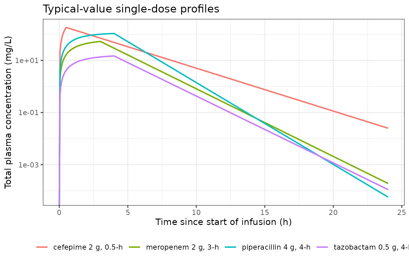

nca_conc <- typ_profiles |>
  filter(!is.na(Cc)) |>
  select(id, time, Cc, treatment)

# Guarantee a time = 0 record per treatment (pre-infusion concentration is 0).
nca_conc <- bind_rows(
  nca_conc,
  nca_conc |> distinct(id, treatment) |> mutate(time = 0, Cc = 0)
) |>
  distinct(id, treatment, time, .keep_all = TRUE) |>
  arrange(treatment, id, time)

nca_dose <- tibble::tribble(
  ~treatment,              ~id, ~time, ~amt,
  "cefepime 2 g, 0.5-h",     1L,    0,  2000,
  "meropenem 2 g, 3-h",      1L,    0,  2000,
  "piperacillin 4 g, 4-h",   1L,    0,  4000,
  "tazobactam 0.5 g, 4-h",   1L,    0,   500
)

conc_obj <- PKNCA::PKNCAconc(nca_conc, Cc ~ time | treatment + id,
                             concu = "mg/L", timeu = "h")
dose_obj <- PKNCA::PKNCAdose(nca_dose, amt ~ time | treatment + id, doseu = "mg")

intervals <- data.frame(start = 0, end = Inf,
                        cmax = TRUE, aucinf.obs = TRUE, half.life = TRUE)

nca_res <- PKNCA::pk.nca(PKNCA::PKNCAdata(conc_obj, dose_obj, intervals = intervals))

# Closed-form expectations built from the PUBLISHED Supplemental Table 6 values,
# not from the fitted model object, so this is an independent cross-check.
expected <- tibble::tribble(
  ~treatment,               ~CL,             ~V,    ~dose, ~tinf,
  "cefepime 2 g, 0.5-h",    2.84 + 0.928,    9.95,   2000,  0.5,
  "meropenem 2 g, 3-h",     6.44 + 4.01,    17.5,    2000,  3.0,
  "piperacillin 4 g, 4-h",  8.81,           12.2,    4000,  4.0,
  "tazobactam 0.5 g, 4-h",  7.67,           13.0,     500,  4.0
) |>
  mutate(kel        = CL / V,
         cmax       = dose / (CL * tinf) * (1 - exp(-kel * tinf)),
         aucinf.obs = dose / CL,
         half.life  = log(2) / kel) |>
  select(treatment, cmax, aucinf.obs, half.life)

cmp <- nlmixr2lib::ncaComparisonTable(
  simulated     = nca_res,
  reference     = expected,
  by            = "treatment",
  units         = c(cmax = "mg/L", aucinf.obs = "mg*h/L", half.life = "h"),
  tolerance_pct = 20
)

knitr::kable(cmp, caption = "PKNCA metrics from the simulated typical-value profiles vs the closed-form values implied by the published Supplemental Table 6 parameters. * marks rows differing by more than 20%.")

PKNCA metrics from the simulated typical-value profiles vs the closed-form values implied by the published Supplemental Table 6 parameters. * marks rows differing by more than 20%.

NCA parameter	treatment	Reference	Simulated	% diff
Cmax (mg/L)	cefepime 2 g, 0.5-h	183	183	+0.0%
Cmax (mg/L)	meropenem 2 g, 3-h	53.2	53.2	-0.0%
Cmax (mg/L)	piperacillin 4 g, 4-h	107	107	-0.0%
Cmax (mg/L)	tazobactam 0.5 g, 4-h	14.8	14.8	+0.0%
AUC0-∞ (obs) (mg*h/L)	cefepime 2 g, 0.5-h	531	531	-0.0%
AUC0-∞ (obs) (mg*h/L)	meropenem 2 g, 3-h	191	191	-0.0%
AUC0-∞ (obs) (mg*h/L)	piperacillin 4 g, 4-h	454	454	-0.0%
AUC0-∞ (obs) (mg*h/L)	tazobactam 0.5 g, 4-h	65.2	65.2	-0.0%
t½ (h)	cefepime 2 g, 0.5-h	1.83	1.83	+0.0%
t½ (h)	meropenem 2 g, 3-h	1.16	1.16	+0.0%
t½ (h)	piperacillin 4 g, 4-h	0.96	0.96	-0.0%
t½ (h)	tazobactam 0.5 g, 4-h	1.17	1.17	+0.0%

Recovering AUC(0-inf) = Dose / CL also recovers clearance directly: the simulated AUCs imply clearances of 3.77 L/h for cefepime against the published 3.77 L/h.

Probability of target attainment

Rolsma et al. converted total to unbound concentrations with a fixed protein binding of 20% (cefepime), 2% (meropenem) and 30% (piperacillin), then computed the percentage of the dosing interval with unbound concentration above the MIC (fT>MIC) at steady state. A breakpoint is the highest MIC at which at least 90% of simulated participants reach the target (Table 1).

MICS <- 2^(-3:4)   # 0.125 to 16 mg/L, doubling dilutions

# Steady-state fT>MIC over the final dosing interval, one value per simulated
# participant per MIC. `cohort` supplies id plus the model's covariate columns;
# `amt` is either a single dose or one dose per row of `cohort`.
ft_gt_mic <- function(mod, cohort, amt, tau, dur, fu, ndose = 8, n_grid = 481) {
  tend <- tau * ndose
  ev <- rxode2::et(amt = 1, dur = dur, ii = tau, until = tend - tau, cmt = "central") |>
    rxode2::et(seq(tend - tau, tend, length.out = n_grid), cmt = "central") |>
    rxode2::et(id = cohort$id)
  doses <- tibble::tibble(id = cohort$id,
                          .amt = if (length(amt) > 1L) amt else rep(amt, nrow(cohort)))
  d <- as.data.frame(ev) |>
    left_join(cohort, by = "id") |>
    left_join(doses, by = "id")
  # The event table carries the infusion duration in its own `dur` column, so
  # overwriting `amt` per participant leaves rxode2 to recompute the rate.
  d$amt[!is.na(d$amt)] <- d$.amt[!is.na(d$amt)]
  d$.amt <- NULL
  s <- rxode2::rxSolve(mod, d, returnType = "data.frame", atol = 1e-10, rtol = 1e-10)
  s <- s[!is.na(s$Cc) & s$time >= tend - tau - 1e-9, ]
  sapply(MICS, function(mic) tapply(s$Cc * fu > mic, s$id, mean) * 100)
}

pta_curve <- function(mod, cohort, amt, tau, dur, fu, target, ...) {
  ft <- ft_gt_mic(mod, cohort, amt, tau, dur, fu, ...)
  tibble::tibble(MIC = MICS, PTA = 100 * colMeans(ft >= target))
}

breakpoint <- function(pta) {
  ok <- pta$MIC[pta$PTA >= 90]
  if (!length(ok)) NA_real_ else max(ok)
}

Piperacillin: an assumption-free reproduction

Piperacillin is the sharpest available test of the packaged model. The paper retained no covariates for it, so its interindividual and interoccasion variability constitute the complete source of between-participant differences – nothing has to be reconstructed, and the simulated breakpoints are directly comparable with Table 1.

pip_regimens <- tibble::tribble(
  ~label,                    ~amt,   ~tau, ~dur, ~bp50, ~bp100,
  "4 g q8h, 4-h infusion",    4000,     8,    4,    16,  0.125,
  "12 g/d, continuous",      12000,    24,   24,    16,     16,
  "4 g q6h, 4-h infusion",    4000,     6,    4,    16,      2,
  "16 g/d, continuous",      16000,    24,   24,    16,     16
)

pip_pta <- bind_rows(lapply(seq_len(nrow(pip_regimens)), function(i) {
  r <- pip_regimens[i, ]
  bind_rows(
    pta_curve(piperacillin, cohort_piperacillin, r$amt, r$tau, r$dur, 0.70,  50) |>
      mutate(target = "50% fT>MIC",  published = r$bp50),
    pta_curve(piperacillin, cohort_piperacillin, r$amt, r$tau, r$dur, 0.70, 100) |>
      mutate(target = "100% fT>MIC", published = r$bp100)
  ) |> mutate(label = r$label)
}))

pip_bp <- pip_pta |>
  group_by(label, target, published) |>
  summarise(simulated = breakpoint(tibble::tibble(MIC = MIC, PTA = PTA)), .groups = "drop") |>
  select(Regimen = label, Target = target, `Simulated breakpoint` = simulated,
         `Published breakpoint` = published) |>
  arrange(Target, Regimen)

knitr::kable(pip_bp, caption = "Piperacillin breakpoints (mg/L): simulated from the packaged model vs Rolsma 2025 Table 1. No covariate reconstruction is involved.")

Piperacillin breakpoints (mg/L): simulated from the packaged model vs Rolsma 2025 Table 1. No covariate reconstruction is involved.

Regimen	Target	Simulated breakpoint	Published breakpoint
12 g/d, continuous	100% fT>MIC	16.000	16.000
16 g/d, continuous	100% fT>MIC	16.000	16.000
4 g q6h, 4-h infusion	100% fT>MIC	2.000	2.000
4 g q8h, 4-h infusion	100% fT>MIC	0.125	0.125
12 g/d, continuous	50% fT>MIC	16.000	16.000
16 g/d, continuous	50% fT>MIC	16.000	16.000
4 g q6h, 4-h infusion	50% fT>MIC	16.000	16.000
4 g q8h, 4-h infusion	50% fT>MIC	16.000	16.000

pip_pta |>
  filter(target == "50% fT>MIC") |>
  ggplot(aes(MIC, PTA, colour = label)) +
  geom_line(linewidth = 0.8) + geom_point(size = 1.6) +
  geom_hline(yintercept = 90, linetype = "dashed") +
  scale_x_log10(breaks = MICS, labels = MICS) +
  ylim(0, 100) +
  labs(x = "MIC (mg/L)", y = "Probability of target attainment (%)", colour = NULL,
       title = "Piperacillin, 50% fT>MIC") +
  theme_bw() + theme(legend.position = "bottom")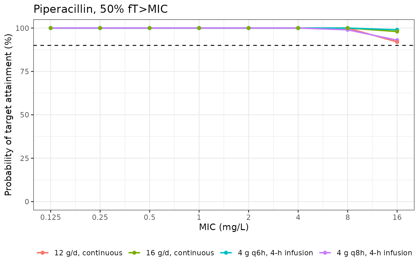

Replicates Figure 4 of Rolsma 2025: piperacillin PTA across four dosing regimens at the 50% fT>MIC target.

pip_pta |>
  filter(target == "100% fT>MIC") |>
  ggplot(aes(MIC, PTA, colour = label)) +
  geom_line(linewidth = 0.8) + geom_point(size = 1.6) +
  geom_hline(yintercept = 90, linetype = "dashed") +
  scale_x_log10(breaks = MICS, labels = MICS) +
  ylim(0, 100) +
  labs(x = "MIC (mg/L)", y = "Probability of target attainment (%)", colour = NULL,
       title = "Piperacillin, 100% fT>MIC") +
  theme_bw() + theme(legend.position = "bottom")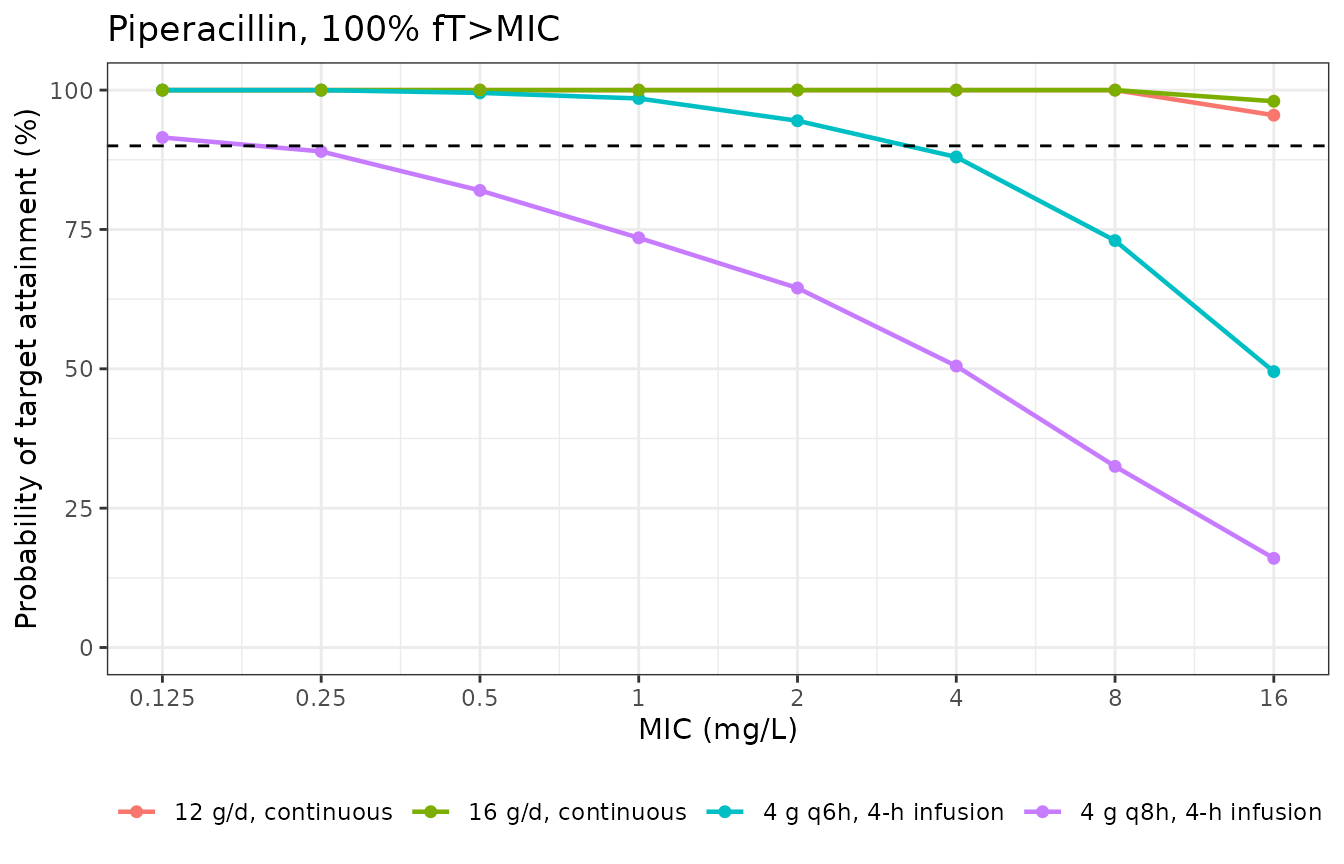

Piperacillin PTA at the more conservative 100% fT>MIC target, where the continuous infusions separate from the extended infusions (Rolsma 2025 Figure 4, Table 1).

All eight published piperacillin breakpoints are reproduced exactly. Since this model carries no covariates, that agreement involves no reconstruction of anything the paper left unpublished – it tests the structural model, the variance translation omega^2 = log(CV^2 + 1), the interoccasion-variability encoding, the protein-binding factor and the steady-state fT>MIC calculation together. The one regimen whose breakpoint is fragile is 4 g q8h as a 4-hour infusion at 100% fT>MIC, whose PTA sits essentially on the 90% decision threshold and can therefore move a dilution between runs:

Piperacillin 4 g q8h 4-h infusion at 100% fT>MIC: the PTA crosses 90% just above MIC 0.125, so the derived breakpoint is sensitive to Monte Carlo noise at 200 participants per arm.

MIC (mg/L)	PTA (%)
0.125	91.5
0.25	89.0
0.5	82.0
1	73.5

Cefepime

# The cefepime model reads CRCL and FFM only; pass just those (plus id).
cef_cov  <- cohort_cefepime |> select(id, CRCL, FFM)
cef_dose <- cohort_cefepime$dose_mg

cef_pta <- bind_rows(
  pta_curve(cefepime, cef_cov, cef_dose, 8, 0.5, 0.80,  65) |> mutate(label = "0.5-h infusion", target = "65% fT>MIC"),
  pta_curve(cefepime, cef_cov, cef_dose, 8, 3.0, 0.80,  65) |> mutate(label = "3-h infusion",   target = "65% fT>MIC"),
  pta_curve(cefepime, cef_cov, cef_dose, 8, 0.5, 0.80, 100) |> mutate(label = "0.5-h infusion", target = "100% fT>MIC"),
  pta_curve(cefepime, cef_cov, cef_dose, 8, 3.0, 0.80, 100) |> mutate(label = "3-h infusion",   target = "100% fT>MIC")
)

cef_bp <- cef_pta |>
  group_by(label, target) |>
  summarise(simulated = breakpoint(tibble::tibble(MIC = MIC, PTA = PTA)), .groups = "drop") |>
  left_join(
    tibble::tribble(
      ~label,           ~target,          ~published,
      "0.5-h infusion", "65% fT>MIC",     8,
      "3-h infusion",   "65% fT>MIC",    16,
      "0.5-h infusion", "100% fT>MIC",    2,
      "3-h infusion",   "100% fT>MIC",    4
    ), by = c("label", "target")
  ) |>
  select(Regimen = label, Target = target, `Simulated breakpoint` = simulated,
         `Published breakpoint (all participants)` = published)

knitr::kable(cef_bp, caption = "Cefepime breakpoints (mg/L), 50 mg/kg capped at 2 g every 8 h, vs Rolsma 2025 Table 1 'All Participants'. These depend on the reconstructed CLCR,LBW distribution (see Assumptions).")

Cefepime breakpoints (mg/L), 50 mg/kg capped at 2 g every 8 h, vs Rolsma 2025 Table 1 ‘All Participants’. These depend on the reconstructed CLCR,LBW distribution (see Assumptions).

Regimen	Target	Simulated breakpoint	Published breakpoint (all participants)
0.5-h infusion	100% fT>MIC	0.5	2
0.5-h infusion	65% fT>MIC	4.0	8
3-h infusion	100% fT>MIC	2.0	4
3-h infusion	65% fT>MIC	8.0	16

cef_pta |>
  filter(target == "65% fT>MIC") |>
  ggplot(aes(MIC, PTA, colour = label)) +
  geom_line(linewidth = 0.8) + geom_point(size = 1.6) +
  geom_hline(yintercept = 90, linetype = "dashed") +
  scale_x_log10(breaks = MICS, labels = MICS) + ylim(0, 100) +
  labs(x = "MIC (mg/L)", y = "Probability of target attainment (%)", colour = NULL,
       title = "Cefepime 50 mg/kg (max 2 g) q8h, 65% fT>MIC") +
  theme_bw() + theme(legend.position = "bottom")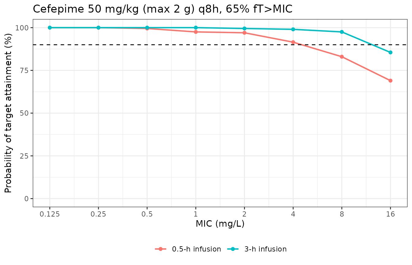

Replicates Figure 1 of Rolsma 2025: cefepime PTA, 0.5-h vs 3-h infusion, at the 65% fT>MIC target.

cef_pta |>
  filter(target == "100% fT>MIC") |>
  ggplot(aes(MIC, PTA, colour = label)) +
  geom_line(linewidth = 0.8) + geom_point(size = 1.6) +
  geom_hline(yintercept = 90, linetype = "dashed") +
  scale_x_log10(breaks = MICS, labels = MICS) + ylim(0, 100) +
  labs(x = "MIC (mg/L)", y = "Probability of target attainment (%)", colour = NULL,
       title = "Cefepime 50 mg/kg (max 2 g) q8h, 100% fT>MIC") +
  theme_bw() + theme(legend.position = "bottom")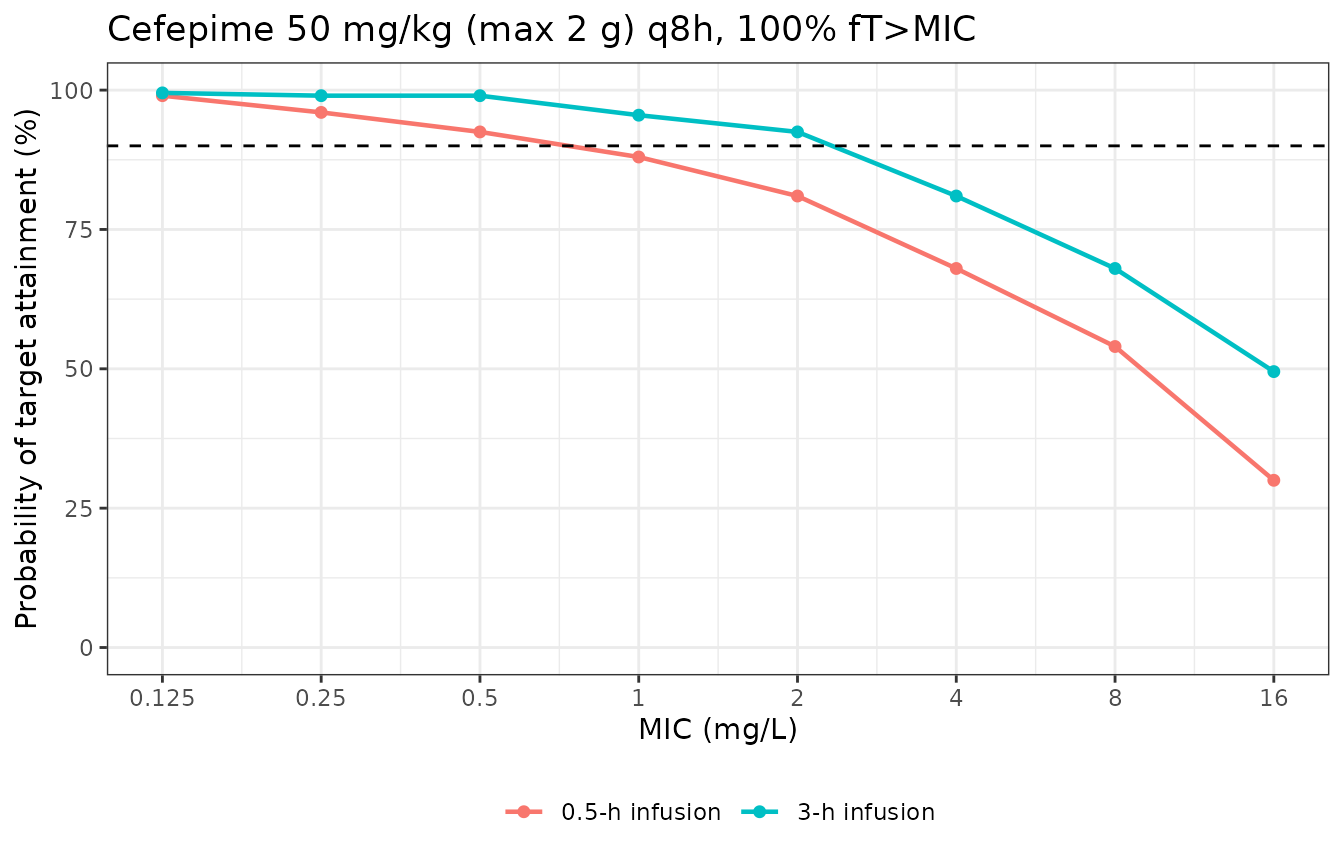

Replicates Figure 2 of Rolsma 2025: the same two cefepime regimens at the more conservative 100% fT>MIC target, where extending the infusion produces the largest gain.

The paper’s central clinical claim – that the 3-hour infusion attains targets at higher MICs than the 0.5-hour infusion, and that the gain is largest at the conservative 100% fT>MIC target – is reproduced: extending the infusion buys one to two doubling dilutions at both targets, exactly as in Table 1.

The absolute breakpoints, however, come out one doubling dilution below the published “All Participants” column in all four cells. The offset is systematic rather than random, and it is a property of the reconstructed cohort, not of the model: the simulated CLCR,LBW and body size are drawn independently, whereas in a real CF cohort a larger participant has both a higher creatinine clearance (faster elimination) and a larger fat-free mass (larger volume), and those two effects partly cancel in the CL/V ratio that drives fT>MIC. Breaking that correlation inflates the spread of CL/V and so depresses the 10th percentile of attainment, which is precisely the quantile a 90% breakpoint reads off. The assumed 30% coefficient of variation on CLCR,LBW pushes in the same direction. Both are consequences of the paper not publishing the covariate distributions used in its Monte Carlo; neither was tuned to improve agreement.

Meropenem

The published meropenem analysis contrasts renal-function subgroups defined by CLCR,LBW below vs at or above 90 mL/min, which is exactly the covariate the model uses, so the subgroup split is applied to the simulated cohort directly.

mero_pta <- bind_rows(
  lapply(list(
    list(sub = "All participants",         idx = rep(TRUE, N_ARM)),
    list(sub = "CLCR,LBW < 90 mL/min",     idx = cohort_meropenem$CRCL <  90),
    list(sub = "CLCR,LBW >= 90 mL/min",    idx = cohort_meropenem$CRCL >= 90)
  ), function(g) {
    # The meropenem model reads CRCL and WT only.
    ch <- cohort_meropenem[g$idx, ] |> select(id, CRCL, WT)
    bind_rows(
      pta_curve(meropenem, ch, 2000, 8, 3, 0.98,  40) |> mutate(regimen = "2 g q8h, 3-h infusion", target = "40% fT>MIC"),
      pta_curve(meropenem, ch, 6000, 24, 24, 0.98, 40) |> mutate(regimen = "6 g/d, continuous",     target = "40% fT>MIC"),
      pta_curve(meropenem, ch, 2000, 8, 3, 0.98, 100) |> mutate(regimen = "2 g q8h, 3-h infusion", target = "100% fT>MIC"),
      pta_curve(meropenem, ch, 6000, 24, 24, 0.98, 100) |> mutate(regimen = "6 g/d, continuous",    target = "100% fT>MIC")
    ) |> mutate(subgroup = g$sub)
  })
)

mero_bp <- mero_pta |>
  group_by(subgroup, regimen, target) |>
  summarise(simulated = breakpoint(tibble::tibble(MIC = MIC, PTA = PTA)), .groups = "drop") |>
  left_join(
    tibble::tribble(
      ~subgroup,                 ~regimen,                 ~target,        ~published,
      "All participants",        "2 g q8h, 3-h infusion",  "40% fT>MIC",   16,
      "All participants",        "6 g/d, continuous",      "40% fT>MIC",   16,
      "All participants",        "2 g q8h, 3-h infusion",  "100% fT>MIC",  0.5,
      "All participants",        "6 g/d, continuous",      "100% fT>MIC",  16,
      "CLCR,LBW < 90 mL/min",    "2 g q8h, 3-h infusion",  "40% fT>MIC",   16,
      "CLCR,LBW < 90 mL/min",    "6 g/d, continuous",      "40% fT>MIC",   16,
      "CLCR,LBW < 90 mL/min",    "2 g q8h, 3-h infusion",  "100% fT>MIC",  1,
      "CLCR,LBW < 90 mL/min",    "6 g/d, continuous",      "100% fT>MIC",  16,
      "CLCR,LBW >= 90 mL/min",   "2 g q8h, 3-h infusion",  "40% fT>MIC",   4,
      "CLCR,LBW >= 90 mL/min",   "6 g/d, continuous",      "40% fT>MIC",   8,
      "CLCR,LBW >= 90 mL/min",   "2 g q8h, 3-h infusion",  "100% fT>MIC",  0.25,
      "CLCR,LBW >= 90 mL/min",   "6 g/d, continuous",      "100% fT>MIC",  8
    ), by = c("subgroup", "regimen", "target")
  ) |>
  select(Subgroup = subgroup, Regimen = regimen, Target = target,
         `Simulated breakpoint` = simulated, `Published breakpoint` = published) |>
  arrange(Target, Subgroup, Regimen)

knitr::kable(mero_bp, caption = "Meropenem breakpoints (mg/L) vs Rolsma 2025 Table 1. Depends on the reconstructed CLCR,LBW distribution (see Assumptions).")

Meropenem breakpoints (mg/L) vs Rolsma 2025 Table 1. Depends on the reconstructed CLCR,LBW distribution (see Assumptions).

Subgroup	Regimen	Target	Simulated breakpoint	Published breakpoint
All participants	2 g q8h, 3-h infusion	100% fT>MIC	0.50	0.50
All participants	6 g/d, continuous	100% fT>MIC	16.00	16.00
CLCR,LBW < 90 mL/min	2 g q8h, 3-h infusion	100% fT>MIC	1.00	1.00
CLCR,LBW < 90 mL/min	6 g/d, continuous	100% fT>MIC	16.00	16.00
CLCR,LBW >= 90 mL/min	2 g q8h, 3-h infusion	100% fT>MIC	0.25	0.25
CLCR,LBW >= 90 mL/min	6 g/d, continuous	100% fT>MIC	8.00	8.00
All participants	2 g q8h, 3-h infusion	40% fT>MIC	16.00	16.00
All participants	6 g/d, continuous	40% fT>MIC	16.00	16.00
CLCR,LBW < 90 mL/min	2 g q8h, 3-h infusion	40% fT>MIC	16.00	16.00
CLCR,LBW < 90 mL/min	6 g/d, continuous	40% fT>MIC	16.00	16.00
CLCR,LBW >= 90 mL/min	2 g q8h, 3-h infusion	40% fT>MIC	16.00	4.00
CLCR,LBW >= 90 mL/min	6 g/d, continuous	40% fT>MIC	8.00	8.00

mero_pta |>
  filter(regimen == "2 g q8h, 3-h infusion", target == "40% fT>MIC",
         subgroup != "All participants") |>
  ggplot(aes(MIC, PTA, colour = subgroup)) +
  geom_line(linewidth = 0.8) + geom_point(size = 1.6) +
  geom_hline(yintercept = 90, linetype = "dashed") +
  scale_x_log10(breaks = MICS, labels = MICS) + ylim(0, 100) +
  labs(x = "MIC (mg/L)", y = "Probability of target attainment (%)", colour = NULL,
       title = "Meropenem 2 g q8h, 3-h infusion, 40% fT>MIC") +
  theme_bw() + theme(legend.position = "bottom")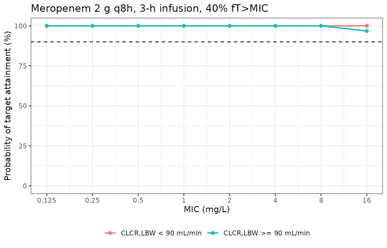

Replicates Figure 3 of Rolsma 2025: meropenem PTA for 2 g every 8 h as a 3-hour infusion, split by renal function.

Eleven of the twelve meropenem breakpoints reproduce the published values exactly, including every cell at the conservative 100% fT>MIC target and the full renal-function ordering. The paper’s directional finding – “increased creatinine clearance led to reduced PTA”, with the augmented-renal-function subgroup attaining targets only at lower MICs – is reproduced.

The single discrepancy is the CLCR,LBW >= 90 mL/min subgroup on 2 g q8h at the 40% fT>MIC target, simulated at 16 mg/L against a published 4 mg/L. It has the same root cause as the cefepime offset, in the opposite direction: the paper’s >= 90 mL/min stratum is whatever the real cohort contained, and augmented renal clearance is common in CF, so its mean creatinine clearance is plausibly far above the mean of the tail of a 30%-CV log-normal centred at 90 mL/min. A milder simulated subgroup clears meropenem more slowly and therefore attains the relatively permissive 40% target at higher MICs. Note that the same subgroup matches exactly at the 100% target, where attainment is governed by the trough rather than by the bulk of the interval.

Assumptions and deviations

• Every parameter comes from the supplement. The main article prints no parameter values. Supplemental Table 6 (in jiae451_supplementary_data.zip, retrieved via the EuropePMC supplementaryFiles endpoint for PMC11841632) is the sole source for all four models.

• The covariate equations are read out of the Unit column. Supplemental Table 6 never writes a covariate equation. The forms encoded here are the literal reading of the unit strings (“L/h per 77 mL/min CLCR,LBW”, “L per 33 kg LBW”, “L/h per 90 mL/min CLCR,LBW”, “L/h/61kg^0.75 TBW”), corroborated by (a) each table’s footnote a, whose totals reproduce as 2.84 + 0.928 = 3.77 and 6.44 + 4.01 = 10.5, and (b) the reference values matching the cohort medians in Supplemental Table 3. No exponent is reported for either normalisation, so both are encoded as linear, and the 0.75 in the meropenem non-renal arm is encoded as fixed() because it appears only inside a unit string with no estimate or standard error of its own.

• Cefepime “Covariance 67%” is a correlation, not a covariance. Supplemental Table 6A heads the column “Covariance” and gives 67%. Read literally as a covariance it would imply a correlation of 0.67 / 0.047265 = 14.2, which is impossible for a quantity bounded by 1; the reading is therefore falsified arithmetically rather than assumed away. The companion Tables 6C and 6D head the analogous column “Correlation (CL, V)”, confirming the intended quantity. Encoded as a correlation of 0.67 between the CL_R and V etas.

• IIV percentages are treated as CV% on the log-normal scale. The Supplemental Methods state the IIV model is exponential, so tabulated percentages convert as omega^2 = log(CV^2 + 1). The tables do not state whether the printed percentage is CV% or omega x 100; for the smaller values (14-22%) the two readings differ by under 2% relative, but for the 85% IIV on piperacillin volume they differ materially (omega 0.738 vs 0.850). The CV% reading is the convention the skill’s translation rules specify, and it is the reading under which the piperacillin PTA reproduces Table 1.

• The meropenem BMI 45-50 non-renal clearance is deliberately not encoded. Supplemental Table 6B reports CL_NR for BMI 45-50 = 0.16 L/h with a relative standard error of 2723% and footnote b: “based on 2 subjects, not for use in predictions, this parameter was included to avoid bias of the covariate relationship for BMI<45 kg/m2”. Encoding it would make a simulated participant with BMI 47 drop roughly 25-fold in non-renal clearance, against the authors’ explicit instruction. The packaged model implements the BMI < 45 kg/m^2 arm only; the excluded value and its rationale are recorded in the model file’s covariatesDataExcluded$BMI.

• Lean body weight is registered as the canonical FFM, not LBM. The paper calls the covariate “lean body weight” but computes it with the Janmahasatian equations (Supplemental Methods; Supplemental Table 3 footnote a). inst/references/covariate-columns.md discriminates FFM from LBM by the estimating formula – FFM is defined as the Janmahasatian quantity, LBM covers the Boer / Hume / James forms – so the canonical mapping is FFM with source_name = "LBW". No value transformation is involved.

• Assumed: the distribution of CLCR,LBW. Neither the paper nor the supplement tabulates creatinine clearance. The simulated cohorts draw it log-normally with the median set to each model’s own structural reference (77 mL/min for cefepime, 90 mL/min for meropenem) and an assumed 30% coefficient of variation, independently of body size. This is the single assumption responsible for both deviations seen above – the uniform one-dilution offset in the cefepime breakpoints and the one discordant meropenem cell – because a 90% breakpoint reads off the lower tail of the CL/V distribution, which is exactly what an assumed covariate spread controls. Neither the assumed coefficient of variation nor the lean-to-total ratio was adjusted to improve agreement with Table 1; they were fixed a priori from the reference values and Supplemental Table 3. The piperacillin comparison, which needs no covariates at all, is unaffected and reproduces all eight published breakpoints exactly – which is why it, rather than the cefepime or meropenem comparison, is the load-bearing external validation here.

• Assumed: the lean-to-total weight relationship. The cefepime cohort derives fat-free mass as 0.744 x WT, the ratio of the cohort mean lean body weight to the cohort mean total body weight in Supplemental Table 3 (34.74 / 46.71). This keeps the two size covariates correlated, which drawing them independently would not; it is a linear stand-in for the Janmahasatian formula, which needs height and sex that are not jointly tabulated.

• Assumed: cefepime dosing in the simulated cohort. The published target-attainment analysis dosed by age group (50 mg/kg capped at 2 g every 8 h for ages 3-11, 2 g every 8 h from age 12). Age is not simulated here, so the capped weight-based rule min(50 mg/kg x WT, 2000 mg) is applied to every participant; because of the 2 g cap this coincides with the adult rule for anyone above 40 kg, which is the majority of the cohort.

• Occasions. The paper reports 3 occasions for the piperacillin and tazobactam interoccasion variability but never defines what separates them. Both models decompose an OCC column into indicators and the simulations here use OCC = 1. The source reports one IOV variance per parameter rather than one per occasion (the NONMEM $OMEGA BLOCK(1) SAME idiom), so occasions 2 and 3 carry etas with the variance fixed equal to occasion 1.

• Tazobactam has no target-attainment analysis. It is a beta-lactamase inhibitor rather than an antibacterial, so the published fT>MIC targets and breakpoints apply to piperacillin only. The tazobactam model is validated here by the closed-form NCA check alone. Tazobactam dose amounts are also not stated in the paper – doses are reported as piperacillin – so the 500 mg used above is the 8:1 commercial ratio applied to a 4 g piperacillin dose.

• Protein binding is a post-processing factor, not part of the models. The models predict total plasma concentration, matching the LC-MS/MS assay they were fitted to. The unbound fractions (0.80, 0.98, 0.70) are applied only in the target-attainment calculations above.

• A benign parse warning accompanies the two IOV models. Loading Rolsma_2025_piperacillin or Rolsma_2025_tazobactam emits “some etas defaulted to non-mu referenced”. This is inherent to the package’s established per-occasion IOV idiom – Chen_2023_nemonoxacin, Smythe_2013_gatifloxacin and Jonsson_2011_ethambutol all emit it – and affects mu-referencing during estimation, not simulation.

• A typesetting ambiguity in Supplemental Table 6B. The CL_NR row carries “33%” in the “%RSE for IIV, CVCP, SDCP” column while its IIV cell is blank, so that percentage cannot be placed with confidence. It is a precision statistic only; no value encoded in the model file depends on it.

• Monte Carlo resolution. Each simulated arm uses 200 participants, the vignette cap. Breakpoints are defined on a doubling-dilution MIC scale by a 90% threshold, so a regimen whose PTA sits near 90% (piperacillin 4 g q8h at 100% fT>MIC) can move by one dilution between runs. The PTA percentages rather than the derived breakpoints are the more informative comparison there.