TMDD approximations for HL2351 and efineptakin alfa (Byun 2024)
Source:vignettes/articles/Byun_2024_tmdd_approximations.Rmd
Byun_2024_tmdd_approximations.Rmd
library(nlmixr2lib)
library(rxode2)
#> rxode2 5.1.8 using 2 threads (see ?getRxThreads)
#>   no cache: create with `rxCreateCache()`
library(dplyr)
#>
#> Attaching package: 'dplyr'
#> The following objects are masked from 'package:stats':
#>
#>     filter, lag
#> The following objects are masked from 'package:base':
#>
#>     intersect, setdiff, setequal, union
library(tidyr)
library(ggplot2)
library(PKNCA)
#>
#> Attaching package: 'PKNCA'
#> The following object is masked from 'package:stats':
#>
#>     filter
Validity of TMDD approximations
Byun 2024 (PLoS Comput Biol 20(4):e1012066, doi:10.1371/journal.pcbi.1012066) asks when the usual simplifications of a target-mediated drug disposition (TMDD) model can stand in for the full binding model. It compares three of them:
- mTMDD – the Michaelis-Menten model obtained with the standard quasi-steady-state approximation (sQSSA);
- qTMDD – the quasi-steady-state model obtained with the total QSSA, where free drug is the positive root of a quadratic in the total drug;
- pTMDD – the paper’s new first-order (Pade) approximation of the qTMDD quadratic, which needs no square root.
It derives validity criteria Lm, Lq and
Lp for each (Table 1), condenses them into a simple rule on
C0 + km versus Rtot (Table 3), and then refits
two clinical Fc-fusion protein datasets with the full model and all
three approximations. Those eight refitted population PK
models (Table 4, with NONMEM control streams in S1 Text) are
what nlmixr2lib ships:
models <- c(
  "Byun_2024_HL2351_tmdd", "Byun_2024_HL2351_mtmdd",
  "Byun_2024_HL2351_qtmdd", "Byun_2024_HL2351_ptmdd",
  "Byun_2024_efineptakin_alfa_tmdd", "Byun_2024_efineptakin_alfa_mtmdd",
  "Byun_2024_efineptakin_alfa_qtmdd", "Byun_2024_efineptakin_alfa_ptmdd"
)
mods <- lapply(setNames(models, models), readModelDb)| Case | Approximation | Model | Observed quantity |
|---|---|---|---|
| 1: HL2351 (hIL-1Ra-hyFc) | TMDD (full) | Byun_2024_HL2351_tmdd | free |
| 1: HL2351 (hIL-1Ra-hyFc) | mTMDD | Byun_2024_HL2351_mtmdd | total |
| 1: HL2351 (hIL-1Ra-hyFc) | qTMDD | Byun_2024_HL2351_qtmdd | free |
| 1: HL2351 (hIL-1Ra-hyFc) | pTMDD | Byun_2024_HL2351_ptmdd | free |
| 2: efineptakin alfa (rhIL-7-hyFc) | TMDD (full) | Byun_2024_efineptakin_alfa_tmdd | free + baseline IL-7 |
| 2: efineptakin alfa (rhIL-7-hyFc) | mTMDD | Byun_2024_efineptakin_alfa_mtmdd | total + baseline IL-7 |
| 2: efineptakin alfa (rhIL-7-hyFc) | qTMDD | Byun_2024_efineptakin_alfa_qtmdd | free + baseline IL-7 |
| 2: efineptakin alfa (rhIL-7-hyFc) | pTMDD | Byun_2024_efineptakin_alfa_ptmdd | free + baseline IL-7 |
Both drugs share one structure (Byun 2024 S1 Text): extravascular depot(s), an FcRn-bearing space in which drug either binds FcRn and is recycled to plasma or is degraded, and target binding (IL1R for HL2351, IL-7R for efineptakin alfa) in the central compartment. The four variants differ only in how the two binding reactions are written:
| Variant | Binding in the FcRn space and in central |
|---|---|
| TMDD | explicit kon, koff with the complex as an
ODE state |
| mTMDD | bound = Rtot * C / (KSS + C), C = state
concentration treated as free |
| qTMDD | free =
0.5 * ((Ct - Rtot - KSS) + sqrt((Ct - Rtot - KSS)^2 + 4 * KSS * Ct))
|
| pTMDD | bound = Rtot * Ct / (KSS + Ct + Rtot), free =
Ct - bound |
Population
Case 1, HL2351. The five HL2351 cohorts (1, 2, 4, 8
and 12 mg/kg single SC doses, n = 8 each) of the first-in-human study
NCT02175056 in healthy adult Korean men, first modelled by Ngo 2020 (doi:10.1002/psp4.12555;
see modellib("Ngo_2020_HL2351")). Byun 2024 does not
restate demographics; age 20-45 years is from Ngo 2020. The S1 Table
dataset has 640 records (40 subjects, 472 observations to 672 h),
matching the 640 stated in the paper.
Case 2, efineptakin alfa. The healthy-subject study
of Lee 2020 (doi:10.1111/cts.12800): single doses of 20 ug/kg SC, 60
ug/kg SC or 60 ug/kg IM (n = 8 each). Byun 2024 reports no demographics.
The S2 Table dataset has 434 records (24 subjects, 410 observations to
672 h) against 456 stated in the paper. The assay measures total serum
IL-7, so each subject’s observed baseline endogenous IL-7
(BL_IL7, 1.51-4.98 pmol/L) is added to the prediction.
Source trace
| Quantity | Source |
|---|---|
| Structural estimates, IIV variances, residual error (all 8 models) | Byun 2024 Table 4 |
| Case 1 Ka2, Alag1, kon1/koff1/kon2/koff2, IIV on Ka2 and Alag1 | S1 Text (a)-(d) $THETA / $OMEGA (not in Table 4) |
| Case 1 FcRn total amount 749 nmol, Vp 5.06 L, Kdeg 0.0264 /h | S1 Text (a)-(d) $THETA, FIX |
| Case 2 VIIM, VISC (route-specific absorption-space volume) | S1 Text (e)-(h) $THETA 13-14 (not in Table 4) |
| Case 2 kon1, koff1, KD, FcRn, FR, kon2, koff2, Kup | S1 Text (e)-(h) $PK hard-coded constants |
| Case 2 KSS1 = KD + Krec / kon1; KSS2 = (Kint + koff2) / kon2 | S1 Text (f)-(h) $PK |
| Compartment order and ODEs | S1 Text (a)-(h) $MODEL and $DES |
| Observation and residual-error model | S1 Text (a)-(h) $ERROR |
| Approximation formulas and validity criteria | Byun 2024 Table 1, Materials and methods |
| Simple validity rule | Byun 2024 Table 3 |
| Generic parameter sets | Byun 2024 Table 2 and Figure 2 legend |
| Datasets (record counts, dose amounts, baseline IL-7) | S1 Table and S2 Table |
Every ini() entry carries an in-file comment naming its
Table 4 cell and the matching $THETA / $OMEGA
index of the control stream.
The approximations on the paper’s generic parameter sets
Before the clinical models, the approximation formulas themselves can
be checked against the paper’s own claims. The chunk below codes the
one-compartment TMDD model with constant total target
(kint = kdeg, Byun 2024 Eq. 1-2) next to the three
approximations of Table 1, and measures each approximation’s maximum
deviation from the full model’s total drug, relative to the full model’s
peak. The approximations are written here directly from Table 1,
independently of the library models.
generic <- rxode2::rxode2({
  km <- (koff + kint) / kon
  dq <- cq - rtot - km
  cqf <- 0.5 * (dq + sqrt(dq * dq + 4 * km * cq))
  d/dt(cf) <- -kel * cf - kon * cf * (rtot - rc) + koff * rc
  d/dt(rc) <- kon * cf * (rtot - rc) - (koff + kint) * rc
  d/dt(cm) <- -kel * cm - kint * rtot * cm / (km + cm)
  d/dt(cq) <- -kel * cqf - kint * rtot * cqf / (km + cqf)
  d/dt(cp) <- -kel * cp - (kint - kel) * rtot * cp / (km + rtot + cp)
  ctot <- cf + rc
})

genericError <- function(kel, kon, koff, kint, rtot, c0, tmax = 48) {
  s <- rxode2::rxSolve(
    generic,
    rxode2::et(seq(0, tmax, length.out = 401)),
    params = c(kel = kel, kon = kon, koff = koff, kint = kint, rtot = rtot),
    inits = c(cf = c0, rc = 0, cm = c0, cq = c0, cp = c0),
    returnType = "data.frame"
  )
  pk <- max(s$ctot)
  c(
    mTMDD = max(abs(s$cm - s$ctot)) / pk,
    qTMDD = max(abs(s$cq - s$ctot)) / pk,
    pTMDD = max(abs(s$cp - s$ctot)) / pk
  )
}
Figure 2: the ratio C0 / Rtot decides
Figure 2 uses kel = 0.05, kon = 0.5,
koff = 0.1, kint = 1, Rtot = 20
(so km = 2.2) and varies C0 / Rtot. The
paper’s reading: at C0 / Rtot = 0.1 qTMDD and pTMDD are
accurate but mTMDD is not; at 1 only qTMDD is accurate; at large ratios
all three are.
fig2 <- lapply(c(0.1, 1, 10, 100), function(r) {
  e <- genericError(kel = 0.05, kon = 0.5, koff = 0.1, kint = 1, rtot = 20, c0 = 20 * r)
  tibble::tibble(ratio = r, model = names(e), error = unname(e))
}) |>
  bind_rows()

fig2 |>
  pivot_wider(names_from = model, values_from = error) |>
  rename("C0 / Rtot" = ratio) |>
knitr::kable(digits = 3, caption = "Maximum relative deviation from the full TMDD model (Figure 2 parameters).")| C0 / Rtot | mTMDD | qTMDD | pTMDD |
|---|---|---|---|
| 0.1 | 0.688 | 0.057 | 0.046 |
| 1.0 | 0.310 | 0.052 | 0.136 |
| 10.0 | 0.045 | 0.005 | 0.092 |
| 100.0 | 0.008 | 0.000 | 0.012 |
err <- function(r, m) fig2$error[fig2$ratio == r & fig2$model == m]
stopifnot(
  # C0 / Rtot = 0.1: qTMDD and pTMDD accurate, mTMDD not
  err(0.1, "qTMDD") < 0.1, err(0.1, "pTMDD") < 0.1, err(0.1, "mTMDD") > 0.1,
  # C0 / Rtot = 1: only qTMDD accurate
  err(1, "qTMDD") < 0.1, err(1, "pTMDD") > 0.1, err(1, "mTMDD") > 0.1,
  # C0 / Rtot = 100: all accurate
  all(fig2$error[fig2$ratio == 100] < 0.1)
)
The three regimes reproduce, which confirms that the pTMDD formula in
Table 1
(dCtot/dt = -kel Ctot - (kint - kel) Rtot Ctot / (km + Rtot + Ctot))
has been read correctly. These are deterministic solves, so the
thresholds are exact.
Table 2 cases and the validity criteria
Table 1’s criteria, evaluated at C0 = 200 for the nine
Table 2 parameter sets, next to the deviations measured as above:
tab2 <- tibble::tibble(
  case = 1:9,
  kon = c(0.1, 0.1, 0.5, 0.1, 0.1, 0.5, 0.1, 0.1, 1e-4),
  koff = c(0.01, 2, 0.5, 0.01, 2, 0.5, 0.01, 2, 0.1),
  kint = c(2, 2, 2, 0.2, 0.2, 0.2, 0.02, 0.02, 3),
  rtot = c(10, 10, 10, 100, 100, 1000, 1000, 1000, 1000),
  kel = 1e-5,
  c0 = 200
) |>
  mutate(
    km = (koff + kint) / kon,
    Lm = kel / (kon * (c0 + km)) + rtot / (c0 + km),
    Lq = kel / (kon * (c0 + km + rtot)) + kint * rtot / (kon * (c0 + km + rtot)^2),
    Lp = Lq + 4 * c0 * rtot / (c0 + rtot + km)^2
  )

errs <- t(mapply(genericError, tab2$kel, tab2$kon, tab2$koff, tab2$kint, tab2$rtot, tab2$c0))
tab2 <- bind_cols(tab2, as.data.frame(errs))

tab2 |>
  select(case, km, Lm, Lq, Lp, mTMDD, qTMDD, pTMDD) |>
  rename("Case" = case, "km" = km, "error mTMDD" = mTMDD, "error qTMDD" = qTMDD, "error pTMDD" = pTMDD) |>
knitr::kable(digits = 3, caption = "Validity criteria (Table 1) and simulated deviations for the Table 2 cases, C0 = 200.")| Case | km | Lm | Lq | Lp | error mTMDD | error qTMDD | error pTMDD |
|---|---|---|---|---|---|---|---|
| 1 | 20.1 | 0.045 | 0.004 | 0.155 | 0.013 | 0.006 | 0.039 |
| 2 | 40.0 | 0.042 | 0.003 | 0.131 | 0.013 | 0.003 | 0.025 |
| 3 | 5.0 | 0.049 | 0.001 | 0.174 | 0.014 | 0.004 | 0.067 |
| 4 | 2.1 | 0.495 | 0.002 | 0.879 | 0.175 | 0.007 | 0.234 |
| 5 | 22.0 | 0.450 | 0.002 | 0.774 | 0.159 | 0.004 | 0.149 |
| 6 | 1.4 | 4.965 | 0.000 | 0.555 | 0.806 | 0.000 | 0.047 |
| 7 | 0.3 | 4.993 | 0.000 | 0.555 | 0.816 | 0.000 | 0.048 |
| 8 | 20.2 | 4.541 | 0.000 | 0.537 | 0.745 | 0.000 | 0.046 |
| 9 | 31000.0 | 0.032 | 0.029 | 0.030 | 0.028 | 0.025 | 0.025 |
km_printed <- c(20, 40, 5, 2, 22, 1.4, 0.2, 20.2, 31000)
km_koff0 <- with(tab2, (ifelse(case %in% c(1, 4, 7), 0, koff) + kint) / kon)
stopifnot(
  # The printed km column is (koff + kint) / kon with the ORIGINAL koff = 0 in
  # cases 1, 4 and 7; the legend's change of koff to 0.01 was not carried into it.
  isTRUE(all.equal(km_koff0, km_printed)),
  !isTRUE(all.equal(tab2$km, km_printed)),
  # qTMDD: Lq < 0.6 and accurate in every case
  all(tab2$Lq < 0.6), all(tab2$qTMDD < 0.1),
  # mTMDD: Lm < 0.1 and accurate exactly in cases 1-3 and 9
  identical(which(tab2$Lm < 0.1), c(1L, 2L, 3L, 9L)),
  identical(which(tab2$mTMDD < 0.1), c(1L, 2L, 3L, 9L)),
  # pTMDD: inaccurate exactly where Lp > 0.6 (cases 4 and 5)
  identical(which(tab2$Lp > 0.6), c(4L, 5L)),
  identical(which(tab2$pTMDD > 0.1), c(4L, 5L))
)
Each criterion separates the accurate cases from the inaccurate ones
exactly. The Results text groups case 6 with cases 4 and 5 as a pTMDD
failure; with the Table 2 values case 6 has Lp = 0.555,
essentially the same as case 7, and its simulated deviation is small, so
this vignette reads case 6 as accurate (see Assumptions and
deviations).
Case 1: HL2351
Parameter cross-check: KSS from the full model
The qTMDD constants are quasi-steady-state combinations of the full
model’s rate constants, so the full TMDD estimates predict them. In
central, KSS2 = (koff2 + Kint) / kon2. In the absorption
space the S1 Text (a) binding flux is
kon1 * (A / V2) * (FcRn - complex) with FcRn as an amount,
which gives KSS1 = V2 * (koff1 + Krec) / kon1 in nmol.
# Byun 2024 Table 4 and S1 Text (a), full TMDD model
kon1 <- 0.249; koff1 <- 0.466; krec <- 0.0346; v2 <- 117
kon2 <- 6.47; koff2 <- 95.4; kint <- 0.206
kss_case1 <- tibble::tibble(
  Constant = c("KSS1 (nmol)", "KSS2 (nmol/L)"),
  `From full TMDD` = c(v2 * (koff1 + krec) / kon1, (koff2 + kint) / kon2),
  `qTMDD (Table 4)` = c(233, 14.1),
  `pTMDD (Table 4)` = c(162, 14.7),
  `mTMDD (Table 4)` = c(5.97, 67.8)
)
knitr::kable(kss_case1, digits = 1, caption = "Case 1 QSS constants implied by the full model against the estimates.")| Constant | From full TMDD | qTMDD (Table 4) | pTMDD (Table 4) | mTMDD (Table 4) |
|---|---|---|---|---|
| KSS1 (nmol) | 235.2 | 233.0 | 162.0 | 6.0 |
| KSS2 (nmol/L) | 14.8 | 14.1 | 14.7 | 67.8 |
The independently estimated qTMDD constants agree with the full model
to within a few percent (233 vs 235 nmol; 14.1 vs 14.8 nmol/L), and so
does the pTMDD KSS2. pTMDD’s KSS1 (162 nmol)
is lower: in the absorption space the dose (hundreds to thousands of
nmol) is of the order of the 749 nmol of FcRn, which is the
C0 ~ Rtot regime where the first-order approximation is
weakest, and the estimate compensates. The mTMDD constants are not
comparable, because its Michaelis-Menten terms act on the total and
absorb the bound fraction.
Typical-value profiles
Doses are converted from mg/kg for a 70 kg subject at 10.31 nmol/mg (molecular weight about 97 kDa).
NMOL_PER_MG <- 1e6 / 97000
case1_doses <- c(1, 2, 4, 8, 12)
case1_grid <- c(seq(0, 24, by = 1), seq(28, 672, by = 4))
case1_approx <- c(tmdd = "TMDD", mtmdd = "mTMDD", qtmdd = "qTMDD", ptmdd = "pTMDD")

case1_typ <- lapply(names(case1_approx), function(a) {
  mod <- rxode2::zeroRe(mods[[paste0("Byun_2024_HL2351_", a)]])
  lapply(case1_doses, function(d) {
    ev <- rxode2::et(amt = d * 70 * NMOL_PER_MG, cmt = "depot", time = 0) |>
      rxode2::et(case1_grid, cmt = "central")
    rxode2::rxSolve(mod, ev, returnType = "data.frame") |>
      mutate(model = case1_approx[[a]], arm = paste(d, "mg/kg"))
  }) |>
    bind_rows()
}) |>
  bind_rows() |>
  mutate(arm = factor(arm, levels = paste(case1_doses, "mg/kg")))
#> ℹ parameter labels from comments will be replaced by 'label()'
#> ℹ omega/sigma items treated as zero: 'etalka1', 'etalka2', 'etalkrec', 'etalkdeg', 'etalcl', 'etalkup', 'etaltlag'
#> ℹ omega/sigma items treated as zero: 'etalka1', 'etalka2', 'etalkrec', 'etalkdeg', 'etalcl', 'etalkup', 'etaltlag'
#> ℹ omega/sigma items treated as zero: 'etalka1', 'etalka2', 'etalkrec', 'etalkdeg', 'etalcl', 'etalkup', 'etaltlag'
#> ℹ omega/sigma items treated as zero: 'etalka1', 'etalka2', 'etalkrec', 'etalkdeg', 'etalcl', 'etalkup', 'etaltlag'
#> ℹ omega/sigma items treated as zero: 'etalka1', 'etalka2', 'etalkrec', 'etalkdeg', 'etalcl', 'etalkup', 'etaltlag'

ggplot(case1_typ, aes(time, Cc, colour = model, linetype = model)) +
  geom_line(linewidth = 0.6) +
  facet_wrap(~arm, scales = "free_y") +
  labs(
    x = "Time (h)", y = "HL2351 (nmol/L)", colour = NULL, linetype = NULL,
    title = "Case 1: typical-value profiles of the four approximations",
    caption = "mTMDD predicts total, the others free, concentration (each as fitted)."
  ) +
  theme_bw()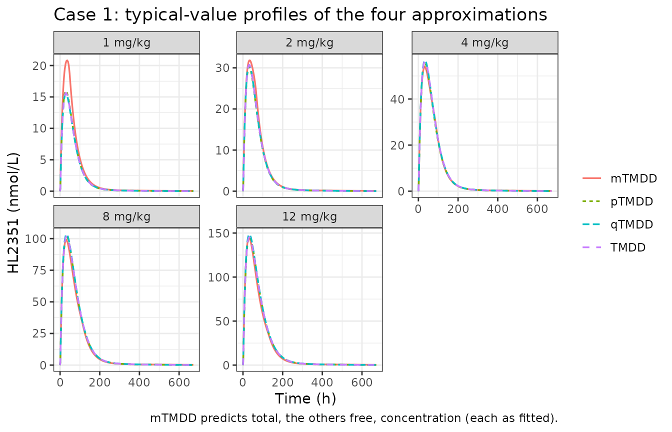
Case 2: efineptakin alfa
Parameter cross-check: the printed KSS values
Table 4 prints KSS1 and KSS2 for the three
approximations although neither is estimated: the control streams
compute them from fixed constants and the estimated Krec.
Recomputing them from the printed inputs:
kd1 <- 29823; kon1_2 <- 4.068e-4
kint_2 <- 0.642; koff2_2 <- 59.76; kon2_2 <- 2.0196e-3
kss_case2 <- tibble::tibble(
  Model = c("mTMDD", "qTMDD", "pTMDD"),
  `Krec (Table 4)` = c(4.68, 0.000602, 0.000619),
  `KSS1 recomputed` = kd1 + `Krec (Table 4)` / kon1_2,
  `KSS1 (Table 4)` = c(41327.42, 29824.48, 29824.52),
  `KSS2 recomputed` = (kint_2 + koff2_2) / kon2_2,
  `KSS2 (Table 4)` = 29007.90
)
knitr::kable(kss_case2, digits = c(0, 6, 2, 2, 1, 2), caption = "Case 2 QSS constants recomputed from the printed inputs.")| Model | Krec (Table 4) | KSS1 recomputed | KSS1 (Table 4) | KSS2 recomputed | KSS2 (Table 4) |
|---|---|---|---|---|---|
| mTMDD | 4.680000 | 41327.42 | 41327.42 | 29907.9 | 29007.9 |
| qTMDD | 0.000602 | 29824.48 | 29824.48 | 29907.9 | 29007.9 |
| pTMDD | 0.000619 | 29824.52 | 29824.52 | 29907.9 | 29007.9 |
stopifnot(
  all(abs(kss_case2$`KSS1 recomputed` - kss_case2$`KSS1 (Table 4)`) < 0.05),
  abs(kss_case2$`KSS2 recomputed`[1] - 29907.9) < 0.1
)
KSS1 reproduces Table 4 to the printed precision, which
also confirms that Table 4’s mTMDD Krec of 4.68 (not the
control stream’s 4.69, which gives 41352) is the final estimate.
KSS2 recomputes to 29907.9, not the printed 29007.90; the
printed value transposes two digits.
Typical-value profiles
Doses are converted from ug/kg for a 70 kg subject at a molecular
weight of 104 kDa (S1 Text (e)); the models apply F = 2 to
express the dose as IL-7 moieties. BL_IL7 is set to zero
here so the profiles show the drug alone.
PMOL_PER_UG <- 1e6 / 104000
case2_arms <- tibble::tibble(
  arm = c("20 ug/kg SC", "60 ug/kg SC", "60 ug/kg IM"),
  ugkg = c(20, 60, 60),
  cmt = c("depot2", "depot2", "depot"),
  ROUTE_SC = c(1, 1, 0)
)
case2_grid <- c(seq(0, 24, by = 1), seq(28, 672, by = 4))

case2_typ <- lapply(names(case1_approx), function(a) {
  mod <- rxode2::zeroRe(mods[[paste0("Byun_2024_efineptakin_alfa_", a)]])
  lapply(seq_len(nrow(case2_arms)), function(i) {
    ev <- rxode2::et(amt = case2_arms$ugkg[i] * 70 * PMOL_PER_UG, cmt = case2_arms$cmt[i], time = 0) |>
      rxode2::et(case2_grid, cmt = "central") |>
      as.data.frame() |>
      mutate(ROUTE_SC = case2_arms$ROUTE_SC[i], BL_IL7 = 0)
    rxode2::rxSolve(mod, ev, returnType = "data.frame") |>
      mutate(model = case1_approx[[a]], arm = case2_arms$arm[i])
  }) |>
    bind_rows()
}) |>
  bind_rows() |>
  mutate(arm = factor(arm, levels = case2_arms$arm))
#> ℹ parameter labels from comments will be replaced by 'label()'
#> ℹ omega/sigma items treated as zero: 'etalq'
#> ℹ omega/sigma items treated as zero: 'etalq'
#> ℹ omega/sigma items treated as zero: 'etalq'
#> ℹ parameter labels from comments will be replaced by 'label()'
#> ℹ omega/sigma items treated as zero: 'etalq'
#> ℹ omega/sigma items treated as zero: 'etalq'
#> ℹ omega/sigma items treated as zero: 'etalq'
#> ℹ parameter labels from comments will be replaced by 'label()'
#> ℹ omega/sigma items treated as zero: 'etalq'
#> ℹ omega/sigma items treated as zero: 'etalq'
#> ℹ omega/sigma items treated as zero: 'etalq'
#> ℹ parameter labels from comments will be replaced by 'label()'
#> ℹ omega/sigma items treated as zero: 'etalq'
#> ℹ omega/sigma items treated as zero: 'etalq'
#> ℹ omega/sigma items treated as zero: 'etalq'

ggplot(case2_typ, aes(time, Cc, colour = model, linetype = model)) +
  geom_line(linewidth = 0.6) +
  facet_wrap(~arm, scales = "free_y") +
  scale_y_log10() +
  labs(
    x = "Time (h)", y = "Efineptakin alfa above baseline (pmol/L IL-7, log scale)",
    colour = NULL, linetype = NULL,
    title = "Case 2: typical-value profiles of the four approximations"
  ) +
  theme_bw()
#> Warning in scale_y_log10(): log-10 transformation introduced infinite values.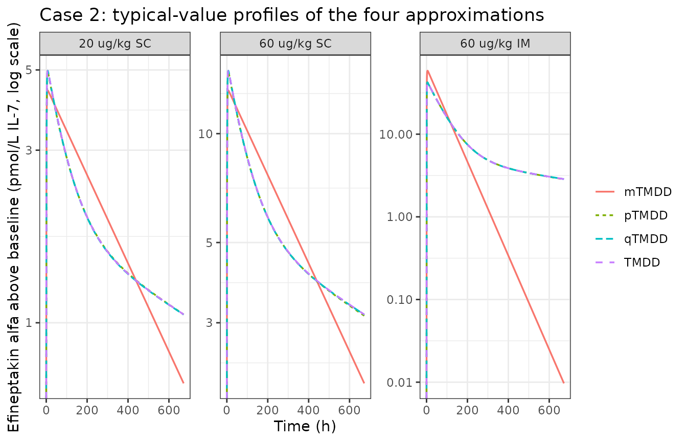
Which regime each case is in
Byun 2024 places case 1 at C0 / Rtot = 22.33 and case 2
at C0 / Rtot = 0.01 without defining C0 for
the clinical data. Taking the typical peak drug concentration as
C0 and the fixed Rtot (2.23 nmol/L and 1060
pmol/L):
regime <- bind_rows(
  case1_typ |> filter(model == "TMDD") |> group_by(arm) |>
    summarise(cmax = max(Cc), .groups = "drop") |> mutate(case = "1: HL2351", rtot = 2.23),
  case2_typ |> filter(model == "TMDD") |> group_by(arm) |>
    summarise(cmax = max(Cc), .groups = "drop") |> mutate(case = "2: efineptakin alfa", rtot = 1060)
) |>
  mutate(ratio = cmax / rtot) |>
  select(case, arm, cmax, rtot, ratio)

regime |>
  rename("Case" = case, "Arm" = arm, "Typical Cmax" = cmax, "Rtot" = rtot, "Cmax / Rtot" = ratio) |>
knitr::kable(digits = 3, caption = "Typical peak drug concentration relative to total target.")| Case | Arm | Typical Cmax | Rtot | Cmax / Rtot |
|---|---|---|---|---|
| 1: HL2351 | 1 mg/kg | 15.654 | 2.23 | 7.020 |
| 1: HL2351 | 2 mg/kg | 30.741 | 2.23 | 13.785 |
| 1: HL2351 | 4 mg/kg | 56.403 | 2.23 | 25.293 |
| 1: HL2351 | 8 mg/kg | 101.755 | 2.23 | 45.630 |
| 1: HL2351 | 12 mg/kg | 145.509 | 2.23 | 65.251 |
| 2: efineptakin alfa | 20 ug/kg SC | 4.975 | 1060.00 | 0.005 |
| 2: efineptakin alfa | 60 ug/kg SC | 14.925 | 1060.00 | 0.014 |
| 2: efineptakin alfa | 60 ug/kg IM | 42.418 | 1060.00 | 0.040 |
stopifnot(
  all(regime$ratio[regime$case == "1: HL2351"] > 5),
  all(regime$ratio[regime$case == "2: efineptakin alfa"] < 0.1)
)
Case 1 sits well above Rtot at every dose (7 to 65; the
paper’s 22.33 falls between the 2 and 4 mg/kg arms), and case 2 at 0.005
to 0.04 of it (the paper’s 0.01 falls between the two SC arms): the two
regimes the paper uses them to represent.
Non-compartmental comparison against the full model
Byun 2024 reports no NCA. Its claim is about agreement between the fitted approximations and the fitted full model: in case 1 all three approximations agree with TMDD, while in case 2 qTMDD and pTMDD agree but mTMDD does not (Table 4 and Figure 3). The NCA below tests that claim on the typical-value profiles, using each case’s full TMDD model as the reference.
nca_conc <- bind_rows(
  case1_typ |> mutate(case = "1"),
  case2_typ |> mutate(case = "2")
) |>
  filter(!is.na(Cc)) |>
  mutate(arm = as.character(arm), id = 1L) |>
  select(case, model, arm, id, time, Cc)

nca_dose <- nca_conc |>
  distinct(case, model, arm, id) |>
  mutate(time = 0, amt = 1)

conc_obj <- PKNCA::PKNCAconc(nca_conc, Cc ~ time | case + model + arm + id)
dose_obj <- PKNCA::PKNCAdose(nca_dose, amt ~ time | case + model + arm + id)
intervals <- data.frame(start = 0, end = 672, cmax = TRUE, tmax = TRUE, auclast = TRUE)
nca_res <- PKNCA::pk.nca(PKNCA::PKNCAdata(conc_obj, dose_obj, intervals = intervals))
nca_tbl <- as.data.frame(nca_res)

nca_ref <- nca_tbl |>
  filter(model == "TMDD") |>
  select(case, arm, PPTESTCD, PPORRES)
nca_approx <- nca_tbl |>
  filter(model != "TMDD") |>
  select(case, model, arm, PPTESTCD, PPORRES)
nca_ref_by_model <- nca_approx |>
  distinct(case, model, arm) |>
  left_join(nca_ref, by = c("case", "arm"), relationship = "many-to-many")

cmp <- ncaComparisonTable(
  simulated = nca_approx,
  reference = nca_ref_by_model,
  by = c("case", "model", "arm"),
  params = c("cmax", "auclast"),
  tolerance_pct = 10
)
knitr::kable(cmp, caption = "Each approximation (Simulated) against the full TMDD model of the same case (Reference).")| NCA parameter | case | model | arm | Reference | Simulated | % diff |
|---|---|---|---|---|---|---|
| Cmax | 1 | mTMDD | 1 mg/kg | 15.7 | 20.8 | +33.0%* |
| Cmax | 1 | mTMDD | 12 mg/kg | 146 | 145 | -0.6% |
| Cmax | 1 | mTMDD | 2 mg/kg | 30.7 | 31.8 | +3.5% |
| Cmax | 1 | mTMDD | 4 mg/kg | 56.4 | 54 | -4.3% |
| Cmax | 1 | mTMDD | 8 mg/kg | 102 | 99 | -2.7% |
| Cmax | 1 | pTMDD | 1 mg/kg | 15.7 | 15.9 | +1.9% |
| Cmax | 1 | pTMDD | 12 mg/kg | 146 | 146 | +0.1% |
| Cmax | 1 | pTMDD | 2 mg/kg | 30.7 | 30.3 | -1.6% |
| Cmax | 1 | pTMDD | 4 mg/kg | 56.4 | 55.7 | -1.2% |
| Cmax | 1 | pTMDD | 8 mg/kg | 102 | 102 | +0.0% |
| Cmax | 1 | qTMDD | 1 mg/kg | 15.7 | 15.6 | -0.6% |
| Cmax | 1 | qTMDD | 12 mg/kg | 146 | 149 | +2.1% |
| Cmax | 1 | qTMDD | 2 mg/kg | 30.7 | 30.7 | -0.2% |
| Cmax | 1 | qTMDD | 4 mg/kg | 56.4 | 56.8 | +0.7% |
| Cmax | 1 | qTMDD | 8 mg/kg | 102 | 103 | +1.6% |
| Cmax | 2 | mTMDD | 20 ug/kg SC | 4.97 | 4.39 | -11.8%* |
| Cmax | 2 | mTMDD | 60 ug/kg IM | 42.4 | 58.6 | +38.1%* |
| Cmax | 2 | mTMDD | 60 ug/kg SC | 14.9 | 13.2 | -11.8%* |
| Cmax | 2 | pTMDD | 20 ug/kg SC | 4.97 | 4.94 | -0.8% |
| Cmax | 2 | pTMDD | 60 ug/kg IM | 42.4 | 42.4 | -0.1% |
| Cmax | 2 | pTMDD | 60 ug/kg SC | 14.9 | 14.8 | -0.8% |
| Cmax | 2 | qTMDD | 20 ug/kg SC | 4.97 | 4.98 | +0.0% |
| Cmax | 2 | qTMDD | 60 ug/kg IM | 42.4 | 42.4 | -0.1% |
| Cmax | 2 | qTMDD | 60 ug/kg SC | 14.9 | 14.9 | +0.0% |
| AUClast | 1 | mTMDD | 1 mg/kg | 1240 | 1580 | +28.0%* |
| AUClast | 1 | mTMDD | 12 mg/kg | 14000 | 13400 | -4.7% |
| AUClast | 1 | mTMDD | 2 mg/kg | 2580 | 2780 | +7.5% |
| AUClast | 1 | mTMDD | 4 mg/kg | 5080 | 4970 | -2.2% |
| AUClast | 1 | mTMDD | 8 mg/kg | 9670 | 9190 | -4.9% |
| AUClast | 1 | pTMDD | 1 mg/kg | 1240 | 1250 | +1.3% |
| AUClast | 1 | pTMDD | 12 mg/kg | 14000 | 14000 | -0.1% |
| AUClast | 1 | pTMDD | 2 mg/kg | 2580 | 2530 | -1.8% |
| AUClast | 1 | pTMDD | 4 mg/kg | 5080 | 4990 | -1.9% |
| AUClast | 1 | pTMDD | 8 mg/kg | 9670 | 9600 | -0.7% |
| AUClast | 1 | qTMDD | 1 mg/kg | 1240 | 1230 | -0.6% |
| AUClast | 1 | qTMDD | 12 mg/kg | 14000 | 14200 | +1.3% |
| AUClast | 1 | qTMDD | 2 mg/kg | 2580 | 2570 | -0.3% |
| AUClast | 1 | qTMDD | 4 mg/kg | 5080 | 5090 | +0.3% |
| AUClast | 1 | qTMDD | 8 mg/kg | 9670 | 9760 | +0.9% |
| AUClast | 2 | mTMDD | 20 ug/kg SC | 1260 | 1350 | +7.3% |
| AUClast | 2 | mTMDD | 60 ug/kg IM | 5710 | 4780 | -16.3%* |
| AUClast | 2 | mTMDD | 60 ug/kg SC | 3780 | 4050 | +7.3% |
| AUClast | 2 | pTMDD | 20 ug/kg SC | 1260 | 1260 | -0.2% |
| AUClast | 2 | pTMDD | 60 ug/kg IM | 5710 | 5710 | -0.1% |
| AUClast | 2 | pTMDD | 60 ug/kg SC | 3780 | 3760 | -0.4% |
| AUClast | 2 | qTMDD | 20 ug/kg SC | 1260 | 1260 | -0.2% |
| AUClast | 2 | qTMDD | 60 ug/kg IM | 5710 | 5710 | -0.0% |
| AUClast | 2 | qTMDD | 60 ug/kg SC | 3780 | 3770 | -0.2% |
* marks a difference above 10%. Case 1 mTMDD predicts
the total concentration, as it was fitted to, so its comparison with the
free-drug TMDD prediction mixes two quantities; its departure is
expected.
pct <- nca_approx |>
  inner_join(nca_ref, by = c("case", "arm", "PPTESTCD"), suffix = c("", "_ref")) |>
  filter(PPTESTCD %in% c("cmax", "auclast")) |>
  mutate(pct_diff = 100 * (PPORRES - PPORRES_ref) / PPORRES_ref)

pct |>
  group_by(case, model) |>
  summarise(max_abs_pct_diff = max(abs(pct_diff)), .groups = "drop") |>
  rename("Case" = case, "Model" = model, "Largest |% diff| (Cmax, AUC)" = max_abs_pct_diff) |>
knitr::kable(digits = 1, caption = "Largest Cmax / AUC(0-672 h) difference from the full model, per approximation.")| Case | Model | Largest |% diff| (Cmax, AUC) |
|---|---|---|
| 1 | mTMDD | 33.0 |
| 1 | pTMDD | 1.9 |
| 1 | qTMDD | 2.1 |
| 2 | mTMDD | 38.1 |
| 2 | pTMDD | 0.8 |
| 2 | qTMDD | 0.2 |
stopifnot(
  # qTMDD and pTMDD reproduce the full model in both cases
  all(abs(pct$pct_diff[pct$model %in% c("qTMDD", "pTMDD")]) < 5),
  # mTMDD fails in case 2: the IM Cmax is far above the full model's
  pct$pct_diff[pct$case == "2" & pct$model == "mTMDD" & pct$arm == "60 ug/kg IM" & pct$PPTESTCD == "cmax"] > 20
)
The two approximations the paper recommends for the low-concentration regime, qTMDD and pTMDD, reproduce the full model to within a few percent in both cases, and mTMDD departs in case 2 as Table 4 and Figure 3 report.
Simulated variability (Figure 3)
Figure 3 shows a visual predictive check per model. Without the
individual data in the package, this section simulates 50 subjects per
arm and model and shows the median and 90% prediction interval. For case
2 the subjects’ BL_IL7 values are resampled from the 24
baselines in the S2 Table dataset.
rxode2::rxSetSeed(20240424)
n_per_arm <- 50

case1_vpc <- lapply(names(case1_approx), function(a) {
  mod <- mods[[paste0("Byun_2024_HL2351_", a)]]
  ev <- lapply(seq_along(case1_doses), function(j) {
    rxode2::et(amt = case1_doses[j] * 70 * NMOL_PER_MG, cmt = "depot", time = 0) |>
      rxode2::et(seq(0, 672, by = 8), cmt = "central") |>
      as.data.frame() |>
      tidyr::crossing(sid = seq_len(n_per_arm)) |>
      mutate(id = (j - 1) * n_per_arm + sid, arm = paste(case1_doses[j], "mg/kg"))
  }) |>
    bind_rows() |>
    select(-sid) |>
    arrange(id, time, desc(evid))
  rxode2::rxSolve(mod, ev, keep = "arm", returnType = "data.frame") |>
    mutate(model = case1_approx[[a]])
}) |>
  bind_rows()
#> ℹ parameter labels from comments will be replaced by 'label()'
#> ℹ parameter labels from comments will be replaced by 'label()'
#> ℹ parameter labels from comments will be replaced by 'label()'
#> ℹ parameter labels from comments will be replaced by 'label()'

case1_vpc |>
  filter(time > 0) |>
  group_by(model, arm, time) |>
  summarise(
    p05 = quantile(sim, 0.05), p50 = median(sim), p95 = quantile(sim, 0.95),
    .groups = "drop"
  ) |>
  mutate(arm = factor(arm, levels = paste(case1_doses, "mg/kg"))) |>
  ggplot(aes(time, p50, colour = model, fill = model)) +
  geom_ribbon(aes(ymin = p05, ymax = p95), alpha = 0.15, colour = NA) +
  geom_line(linewidth = 0.6) +
  facet_wrap(~arm, scales = "free_y") +
  scale_y_log10() +
  labs(
    x = "Time (h)", y = "HL2351 (nmol/L, log scale)", colour = NULL, fill = NULL,
    title = "Case 1: median and 90% prediction interval"
  ) +
  theme_bw()
#> Warning in transformation$transform(x): NaNs produced
#> Warning in scale_y_log10(): log-10 transformation introduced infinite values.
#> Warning in transformation$transform(x): NaNs produced
#> Warning in scale_y_log10(): log-10 transformation introduced infinite values.
#> Warning in transformation$transform(x): NaNs produced
#> Warning in scale_y_log10(): log-10 transformation introduced infinite values.
#> Warning: Removed 754 rows containing missing values or values outside the scale range
#> (`geom_ribbon()`).
#> Warning: Removed 2 rows containing missing values or values outside the scale range
#> (`geom_line()`).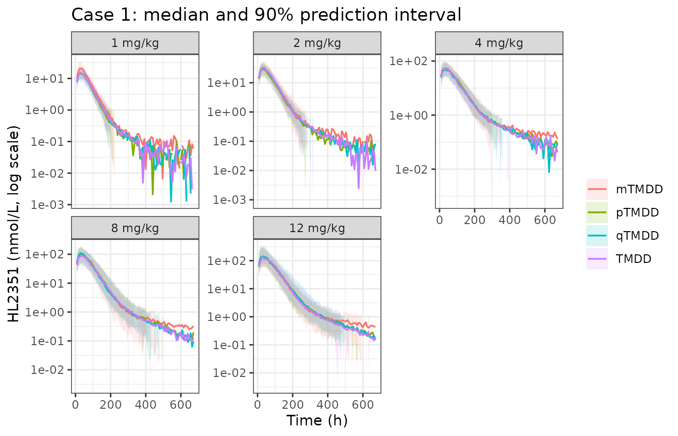
# Per-subject baseline serum IL-7 (pmol/L), Byun 2024 S2 Table, subjects 1-24.
bl_il7_obs <- c(
  2.341463415, 3.804878049, 2.390243902, 1.853658537, 2.146341463, 3.463414634,
  1.512195122, 3.414634146, 4.097560976, 2.243902439, 3.365853659, 2.146341463,
  2.634146341, 4.926829268, 2.585365854, 3.219512195, 4.829268293, 1.756097561,
  4.195121951, 2, 1.658536585, 4.43902439, 4.975609756, 3.170731707
)

case2_ev <- lapply(seq_len(nrow(case2_arms)), function(j) {
  rxode2::et(amt = case2_arms$ugkg[j] * 70 * PMOL_PER_UG, cmt = case2_arms$cmt[j], time = 0) |>
    rxode2::et(c(seq(0, 24, by = 2), seq(32, 672, by = 8)), cmt = "central") |>
    as.data.frame() |>
    tidyr::crossing(sid = seq_len(n_per_arm)) |>
    mutate(id = (j - 1) * n_per_arm + sid, arm = case2_arms$arm[j], ROUTE_SC = case2_arms$ROUTE_SC[j])
}) |>
  bind_rows() |>
  select(-sid) |>
  arrange(id, time, desc(evid))
case2_bl <- tibble::tibble(
  id = sort(unique(case2_ev$id)),
  BL_IL7 = sample(bl_il7_obs, length(unique(case2_ev$id)), replace = TRUE)
)
case2_ev <- left_join(case2_ev, case2_bl, by = "id")

case2_vpc <- lapply(names(case1_approx), function(a) {
  mod <- mods[[paste0("Byun_2024_efineptakin_alfa_", a)]]
  rxode2::rxSolve(mod, case2_ev, keep = "arm", returnType = "data.frame") |>
    mutate(model = case1_approx[[a]])
}) |>
  bind_rows()
#> ℹ parameter labels from comments will be replaced by 'label()'
#> ℹ parameter labels from comments will be replaced by 'label()'
#> ℹ parameter labels from comments will be replaced by 'label()'
#> ℹ parameter labels from comments will be replaced by 'label()'

case2_vpc |>
  filter(time > 0) |>
  group_by(model, arm, time) |>
  summarise(
    p05 = quantile(sim, 0.05), p50 = median(sim), p95 = quantile(sim, 0.95),
    .groups = "drop"
  ) |>
  mutate(arm = factor(arm, levels = case2_arms$arm)) |>
  ggplot(aes(time, p50, colour = model, fill = model)) +
  geom_ribbon(aes(ymin = p05, ymax = p95), alpha = 0.15, colour = NA) +
  geom_line(linewidth = 0.6) +
  facet_grid(model ~ arm, scales = "free_y") +
  scale_y_log10() +
  labs(
    x = "Time (h)", y = "Serum IL-7 (pmol/L, log scale)", colour = NULL, fill = NULL,
    title = "Case 2: median and 90% prediction interval, baseline included"
  ) +
  theme_bw() +
  theme(legend.position = "none")
#> Warning in transformation$transform(x): NaNs produced
#> Warning in scale_y_log10(): log-10 transformation introduced infinite values.
#> Warning: Removed 7 rows containing missing values or values outside the scale range
#> (`geom_ribbon()`).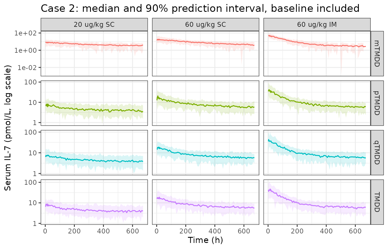
The case 2 mTMDD interval is far wider than the others: its fit put an IIV variance of 13.2 on Q (against 0.29 for the other three), one more symptom of the misfit the paper reports for that approximation.
Assumptions and deviations
-
Table 4 governs the values; the control streams govern the
structure. The S1 Text
$THETA/$OMEGAblocks hold the final estimates re-used as starting values; they agree with Table 4 to within rounding (largest difference: case 2 qTMDD SC absorption rate, 0.697 in Table 4 vs 0.672 in the stream). Quantities that Table 4 does not print are taken from the streams: case 1Ka2,Alag1,kon1,koff1,kon2,koff2and the IIVs onKa2andAlag1; case 2VIIMandVISC. -
Table 4 prints the case 1
Kdegas 0.264. All four control streams fix it at 0.0264 /h, as does Ngo 2020 Table 1; 0.0264 is used. -
Table 4 prints the case 2
KSS2as 29007.90. The streams compute it as(Kint + koff2) / kon2= 29907.9 pmol/L (see the cross-check above); the models compute it the same way. -
Table 4’s legend swaps
KSS1andKSS2(it callsKSS1the drug-target andKSS2the drug-FcRn constant) and describesVdas the peripheral volume andKintas the FcRn-complex internalisation rate. In the control streams, and in these models,KSS1is the FcRn constant,KSS2the target constant,Vdthe volume of the FcRn space, andKintthe loss of the drug-target complex. Table 4’s additive-error unit (pmol/L) applies to case 2; case 1 works in nmol/L. -
The absorption space of case 1 is
abs_site, as in the Ngo 2020 and Jung 2023 HL2351 models. In case 2 the drug reaches the FcRn space only by uptake from the interstitial/vascular space, so that space isendosomeand the interstitial/vascular one isisf. -
Case 2 sets
Kupto 0 whenTIMEis 0 (IF(TIME.EQ.0) Kup=0). NONMEM applies the parameters computed on a record over the interval that ends at that record, so this changes only the empty interval up to time 0. It is not reproduced. -
Route in case 2. The dataset
COHORT(1 = SC 20, 2 = SC 60, 3 = IM 60 ug/kg) selects the volume of the absorption space; it is encoded asROUTE_SC(1 = SC). IM doses go todepotand SC doses todepot2. -
Case 2 mTMDD degrades the whole endosomal amount
(
Kdeg * A(5)), whereas qTMDD and pTMDD degrade only the free amount; this follows the control streams. - Record counts. Case 2’s dataset has 434 records against the 456 stated in the paper.
-
C0is not defined for the clinical data. The regime check above uses the typical peak concentration; that the paper’s 22.33 and 0.01 both fall inside the simulated per-arm ranges suggests a comparable definition (for example a mid-range dose), but this is an inference. -
Table 2’s
kmcolumn useskoff = 0in cases 1, 4 and 7. The legend sayskoffwas changed from 0 to 0.01 in those cases, but the printedkm(20, 2 and 0.2) iskint / kon; withkoff = 0.01it is 20.1, 2.1 and 0.3. The calculations here usekoff = 0.01and thekmit implies; the criteria and the accuracy pattern are the same either way. -
Figure 1 grouping of case 6. The text lists case 6
with cases 4 and 5 as a pTMDD failure. From the Table 2 values case 6
has
Lpof about 0.55, below the paper’s 0.6 threshold and equal to case 7’s, and the generic simulation shows a small pTMDD deviation. The vignette follows the criterion. - Illustrative dosing. All simulations use a 70 kg subject for the weight-based doses; the datasets themselves dose by actual body weight.
- Demographics. Byun 2024 reports none; case 1’s are from Ngo 2020, and none are available for case 2.