Epoetin delta (Knebel 2008)
Source:vignettes/articles/Knebel_2008_epoetinDelta.Rmd
Knebel_2008_epoetinDelta.RmdModel and source
ui <- rxode2::rxode(readModelDb("Knebel_2008_epoetinDelta"))
#> ℹ parameter labels from comments will be replaced by 'label()'- Citation: Knebel W, Palmen M, Dowell JA, Gastonguay M. Population pharmacokinetic modeling of epoetin delta in pediatric patients with chronic kidney disease. J Clin Pharmacol. 2008;48(7):837-848. doi:10.1177/0091270008318218
- Description: One-compartment population PK model with first-order absorption and linear elimination for subcutaneous and intravenous epoetin delta in pediatric patients aged 1-17 years with chronic kidney disease (Knebel 2008). Serum erythropoietin is the sum of the drug contribution and an additive endogenous baseline concentration. Clearance and central volume are allometrically scaled by body weight (exponents 0.75 and 1) about a 35 kg reference, with additional power effects of age above 10 years, a sex factor on both, and dialysis-modality factors on volume. The same model was fit jointly to epoetin alfa data, which enters through a product indicator that shifts the absorption rate constant and the subcutaneous bioavailability.
- Article: https://doi.org/10.1177/0091270008318218
Epoetin delta (Dynepo) is a recombinant human erythropoietin produced
in a human cell line by activation of the endogenous erythropoietin
gene, rather than in Chinese hamster ovary (CHO) cells as every other
erythropoiesis-stimulating agent is. Knebel 2008 is the first population
PK analysis of the product in children. The same NONMEM run also carried
the epoetin alfa arm of the trial, so a single model file holds both
products and a binary product indicator (FORM_EPO_ALFA)
shifts the two subcutaneous absorption parameters.
Population
The analysis dataset was a phase III, open-label, randomized, stratified, multicenter 24-week trial in 60 pediatric patients aged 1 to 17 years with chronic kidney disease and associated anemia, contributing 261 serum erythropoietin concentrations (Knebel 2008 Results). Patients were randomized approximately 3:1 to epoetin delta (47 subjects: 37 subcutaneous, 10 intravenous) or epoetin alfa (13 subjects: 12 subcutaneous, 1 intravenous), at whatever dose and frequency (once, twice, or three times weekly) they had been receiving before consent, titrated to keep hemoglobin in a 10-13 g/dL target range (Table I and Study Design).
Baseline demographics (Table II): weight median 34.5 kg (range 11.3-83), age median 13 years (range 1-17), body surface area median 1.17 m^2 (range 0.506-1.95), body mass index median 17.2 kg/m^2 (range 12.3-28.6). Thirty-eight of 60 subjects (63%) were male. Race was 54 White (90%), 2 African American (3%), 4 multiracial (7%); the two smaller strata were too sparse for formal comparison, so race is not a covariate in the model. Renal replacement status was 28 hemodialysis (47%), 15 peritoneal dialysis (25%), and 17 predialysis (28%).
Two features of the cohort shape the model directly. First, weight,
BSA, BMI, and age were mutually correlated at r >= 0.71 (except
BSA-BMI, r = 0.59, and age-BMI, r = 0.33), so weight was retained as the
single body-size metric. Second, every patient was already stabilized on
an erythropoiesis-stimulating agent at entry, which left too little
between-subject spread in baseline erythropoietin to estimate a
subject-specific baseline – hence a single population Bepo
with no inter-individual variability.
The same information is available programmatically from the model metadata:
str(ui$population, max.level = 1)
#> List of 15
#>  $ species         : chr "human"
#>  $ n_subjects      : int 60
#>  $ n_studies       : int 1
#>  $ n_concentrations: int 261
#>  $ age_range       : chr "1-17 years"
#>  $ age_median      : chr "13 years"
#>  $ weight_range    : chr "11.3-83 kg"
#>  $ weight_median   : chr "34.5 kg"
#>  $ sex_female_pct  : num 37
#>  $ race_ethnicity  : Named num [1:3] 90 3 7
#>   ..- attr(*, "names")= chr [1:3] "White" "African American" "Multiracial"
#>  $ disease_state   : chr "Pediatric chronic kidney disease with associated anemia. Knebel 2008 Table II: 28 subjects (47%) on hemodialysi"| __truncated__
#>  $ dose_range      : chr "Epoetin delta: 26-191 IU/kg subcutaneous (37 subjects), 54-769 IU/kg intravenous (10 subjects). Epoetin alfa: 2"| __truncated__
#>  $ regions         : chr "United States and Argentina (per the ethics-committee appendix of Knebel 2008)"
#>  $ body_size       : chr "Knebel 2008 Table II also reports body mass index (median 17.2, mean 18.1, range 12.3-28.6 kg/m^2) and body sur"| __truncated__
#>  $ notes           : chr "Phase III, open-label, randomized, stratified, multicenter 24-week study of epoetin delta (Dynepo). Sparse samp"| __truncated__
Source trace
Every ini() entry in
inst/modeldb/specificDrugs/Knebel_2008_epoetinDelta.R
carries an in-file comment naming its origin. They are collected here
for review. All parameter values are the Final Model
column of Knebel 2008 Table III; the base-model column of the same table
is a nested precursor with a 70 kg allometric reference (Table III
footnote a) and is not extracted.
| Equation / parameter | Value | Source location |
|---|---|---|
| Structure: 1 compartment, first-order absorption, linear elimination, additive baseline | n/a | Results, “Population Pharmacokinetic Modeling Results” |
IIV form P_i = P * exp(eta_i)
|
n/a | Methods equation (1) |
Residual form C_ij = Chat_ij * exp(eps_ij)
|
n/a | Methods equation (2) |
Allometric form
TVP = theta * (WT/WTref)^theta_allo
|
n/a | Methods equation (3) |
| Power / exponentiated-switch covariate form | n/a | Methods equation (4) |
lcl (CL) |
0.268 L/h | Table III final model, theta1 (35% SE; 95% CI 0.148, 0.827) |
lvc (V) |
1.03 L | Table III final model, theta2 (45% SE; 95% CI 0.344, 6.44) |
lka (Ka, epoetin delta) |
0.0554 1/h | Table III final model, theta3 (16% SE; 95% CI 0.0405, 0.199) |
lfdepot (F1, epoetin delta) |
0.708 | Table III final model, theta4 (38% SE; 95% CI 0.337, 2.12) |
lrbase (Bepo) |
6.71 mIU/mL | Table III final model, theta5 (7% SE; 95% CI 5.72, 7.70) |
e_wt_cl |
0.75, fixed | Results and equation (3); Table III row *(WT/35)^0.75
shows NA in every estimate column |
e_wt_vc |
1, fixed | Results and equation (3); Table III row *(WT/35)^1
shows NA in every estimate column |
e_age_cl |
0.999 | Table III final model, theta8 (54% SE; 95% CI -0.0690, 2.1) |
e_sexf_cl |
0.923 | Table III final model, theta9 (18% SE; 95% CI 0.594, 1.32) |
e_age_vc |
2.89 | Table III final model, theta13 (29% SE; 95% CI 0.0281, 4.95) |
e_sexf_vc |
0.994 | Table III final model, theta10 (39% SE; 95% CI 0.370, 2.31) |
e_hemodial_vc |
4.53 | Table III final model, theta11 (45% SE; 95% CI 1.65, 16.5) |
e_perit_dial_vc |
2.48 | Table III final model, theta12 (39% SE; 95% CI 1.08, 6.13) |
e_epoalfa_ka |
1.23 | Table III final model, theta6 (14% SE; 95% CI 0.495, 1.62); Results quotes relative Ka = 123% |
e_epoalfa_fdepot |
0.544 | Table III final model, theta7 (19% SE; 95% CI 0.368, 0.824); Results quotes relative F1 = 54.4% |
etalcl |
0.387 | Table III final model, Omega(1,1) (29% SE; CV% = 62.2; 95% CI 0.184, 0.671) |
etalvc |
1.41 | Table III final model, Omega(2,2) (33% SE; CV% = 119; 95% CI 0.481, 2.51) |
expSd |
sqrt(0.245) = 0.49497 | Table III final model, sigma(1,1) = 0.245 (13% SE; CV% = 49.5; 95% CI 0.184, 0.308) |
| Reference weight 35 kg | n/a | Results, “The weight normalization … was 35 kg for the full covariate model” |
| Reference age 10 years, hinge above it | n/a | Results, “normalized by the reference age of 10 years for all patients older than 10 years of age” |
| Reference individual: 35 kg male, <= 10 y, predialysis, SC epoetin delta | n/a | Abstract and Results |
Variance versus standard deviation
Table III labels its random-effect blocks “Interindividual Variance”
and “Residual Variance” and prints a CV% line beneath each
entry. The CV% values are the plain square roots of the
tabulated numbers, not the log-normal
sqrt(exp(omega^2) - 1), which is what fixes the tabulated
numbers as variances rather than standard deviations:
c(
  omega_cl_sqrt = sqrt(0.387),  # Table III prints CV% = 62.2
  omega_v_sqrt  = sqrt(1.41),   # Table III prints CV% = 119
  sigma_sqrt    = sqrt(0.245)   # Table III prints CV% = 49.5
)
#> omega_cl_sqrt  omega_v_sqrt    sigma_sqrt
#>     0.6220932     1.1874342     0.4949747

# Had the entries been standard deviations, the printed CV% would have to be
# these instead -- none of which match the table.
c(
  omega_cl_alt = sqrt(exp(0.387^2) - 1),
  omega_v_alt  = sqrt(exp(1.41^2) - 1),
  sigma_alt    = sqrt(exp(0.245^2) - 1)
)
#> omega_cl_alt  omega_v_alt    sigma_alt
#>    0.4019526    2.5103082    0.2487229

stopifnot(
  abs(sqrt(0.387) - 0.622) < 5e-4,
  abs(sqrt(1.41)  - 1.19)  < 5e-3,
  abs(sqrt(0.245) - 0.495) < 5e-4
)
So etalcl ~ 0.387 and etalvc ~ 1.41 go into
ini() unchanged, and expSd is
sqrt(0.245).
Structural checks against the closed form
The model is a one-compartment system with first-order absorption, so the typical-value prediction has a closed form. Comparing the solved profile against it is a tight gate: both sides use the same parameter values, so the only difference is integrator error and a bound of a few parts per million is correct here (unlike the cohort-level checks further down, where per-subject random effects make extreme-value bounds irreproducible across rxode2 builds).
mod  <- readModelDb("Knebel_2008_epoetinDelta")
modz <- rxode2::zeroRe(rxode2::rxode(mod))
#> ℹ parameter labels from comments will be replaced by 'label()'

# Reference individual of Knebel 2008: 35 kg male, age <= 10 years,
# predialysis, subcutaneous epoetin delta.
ref_cov <- list(
  WT = 35, AGE = 5, SEXF = 0,
  RRT_HEMODIAL_STATUS = 0, PERIT_DIAL = 0, FORM_EPO_ALFA = 0
)

# 100 IU/kg is mid-range for the subcutaneous arms (Table I: 26-191 IU/kg).
dose_iu <- 100 * ref_cov$WT

build_events <- function(cov, amt, cmt, times) {
  dosing <- data.frame(
    id = 1L, time = 0, amt = amt, evid = 1L, cmt = cmt
  )
  obs <- data.frame(
    id = 1L, time = times, amt = NA_real_, evid = 0L, cmt = "central"
  )
  out <- dplyr::bind_rows(dosing, obs)
  for (nm in names(cov)) out[[nm]] <- cov[[nm]]
  dplyr::arrange(out, .data$time, dplyr::desc(.data$evid))
}

obs_times <- seq(0, 240, by = 0.25)
ev_ref <- build_events(ref_cov, dose_iu, "depot", obs_times)
sim_ref <- rxode2::rxSolve(modz, ev_ref, returnType = "data.frame")
#> ℹ omega/sigma items treated as zero: 'etalcl', 'etalvc'

# Closed form: one compartment, first-order input, plus the additive endogenous
# baseline. Parameter values read straight off Table III.
cl <- 0.268; vc <- 1.03; ka <- 0.0554; f1 <- 0.708; bepo <- 6.71
kel <- cl / vc
cc_analytic <- f1 * dose_iu / vc * ka / (ka - kel) *
  (exp(-kel * sim_ref$time) - exp(-ka * sim_ref$time)) + bepo

rel_err <- abs(sim_ref$Cc - cc_analytic) / cc_analytic
sprintf("max relative deviation from the closed form: %.2e", max(rel_err))
#> [1] "max relative deviation from the closed form: 3.20e-08"
stopifnot(max(rel_err) < 1e-6)
Two further identities hold exactly and are worth pinning:
# 1. The endogenous baseline is the prediction at time zero for an
#    extravascular dose, and holds forever if no dose is given.
ev_nodose <- build_events(ref_cov, 0, "depot", obs_times)
sim_nodose <- rxode2::rxSolve(modz, ev_nodose, returnType = "data.frame")
#> ℹ omega/sigma items treated as zero: 'etalcl', 'etalvc'
stopifnot(max(abs(sim_nodose$Cc - bepo)) < 1e-10)

# 2. Absorption is rate-limiting: ka (0.0554/h) is well below kel (0.260/h), so
#    the model is in flip-flop and the TERMINAL slope is ka, not kel. This is
#    what makes the published subcutaneous half-life several-fold the
#    intravenous one (Knebel 2008 Introduction, on the adult study).
stopifnot(ka < kel)
c(
  t_half_terminal_sc_h = log(2) / ka,
  t_half_iv_h          = log(2) / kel,
  ratio                = kel / ka
)
#> t_half_terminal_sc_h          t_half_iv_h                ratio
#>            12.511682             2.663961             4.696646
Covariate-model checks
Each covariate term is an exact algebraic factor on cl
or vc, which rxode2 returns as columns of the solve.
Recovering each published coefficient from the ratio of two
typical-value solves confirms the encoding, including the age hinge,
which is the one non-obvious piece of the covariate model.
param_at <- function(...) {
  cov <- utils::modifyList(ref_cov, list(...))
  ev <- build_events(cov, dose_iu, "depot", c(0, 1))
  s <- rxode2::rxSolve(modz, ev, returnType = "data.frame")
  c(cl = s$cl[1], vc = s$vc[1], ka = s$ka[1], fdepot = s$fdepot[1])
}

p_ref <- param_at()
#> ℹ omega/sigma items treated as zero: 'etalcl', 'etalvc'

covariate_checks <- dplyr::bind_rows(
  # Allometric exponents, fixed at 0.75 and 1 about the 35 kg reference.
  tibble::tibble(
    quantity  = "CL exponent on (WT/35)",
    published = 0.75,
    recovered = log(param_at(WT = 70)[["cl"]] / p_ref[["cl"]]) / log(70 / 35)
  ),
  tibble::tibble(
    quantity  = "Vc exponent on (WT/35)",
    published = 1,
    recovered = log(param_at(WT = 70)[["vc"]] / p_ref[["vc"]]) / log(70 / 35)
  ),
  # Age enters only above the 10-year reference: a 15-year-old differs from the
  # reference by (15/10)^theta, while a 5-year-old does not differ at all.
  tibble::tibble(
    quantity  = "CL exponent on (AGE/10), age > 10 y",
    published = 0.999,
    recovered = log(param_at(AGE = 15)[["cl"]] / p_ref[["cl"]]) / log(15 / 10)
  ),
  tibble::tibble(
    quantity  = "Vc exponent on (AGE/10), age > 10 y",
    published = 2.89,
    recovered = log(param_at(AGE = 15)[["vc"]] / p_ref[["vc"]]) / log(15 / 10)
  ),
  # Exponentiated switches: the factor itself is the published theta.
  tibble::tibble(
    quantity  = "CL factor, female",
    published = 0.923,
    recovered = param_at(SEXF = 1)[["cl"]] / p_ref[["cl"]]
  ),
  tibble::tibble(
    quantity  = "Vc factor, female",
    published = 0.994,
    recovered = param_at(SEXF = 1)[["vc"]] / p_ref[["vc"]]
  ),
  tibble::tibble(
    quantity  = "Vc factor, hemodialysis vs predialysis",
    published = 4.53,
    recovered = param_at(RRT_HEMODIAL_STATUS = 1)[["vc"]] / p_ref[["vc"]]
  ),
  tibble::tibble(
    quantity  = "Vc factor, peritoneal dialysis vs predialysis",
    published = 2.48,
    recovered = param_at(PERIT_DIAL = 1)[["vc"]] / p_ref[["vc"]]
  ),
  tibble::tibble(
    quantity  = "Ka factor, epoetin alfa vs delta",
    published = 1.23,
    recovered = param_at(FORM_EPO_ALFA = 1)[["ka"]] / p_ref[["ka"]]
  ),
  tibble::tibble(
    quantity  = "F1 factor, epoetin alfa vs delta",
    published = 0.544,
    recovered = param_at(FORM_EPO_ALFA = 1)[["fdepot"]] / p_ref[["fdepot"]]
  )
) |>
  dplyr::mutate(abs_diff = abs(.data$recovered - .data$published))
#> ℹ omega/sigma items treated as zero: 'etalcl', 'etalvc'
#> ℹ omega/sigma items treated as zero: 'etalcl', 'etalvc'
#> ℹ omega/sigma items treated as zero: 'etalcl', 'etalvc'
#> ℹ omega/sigma items treated as zero: 'etalcl', 'etalvc'
#> ℹ omega/sigma items treated as zero: 'etalcl', 'etalvc'
#> ℹ omega/sigma items treated as zero: 'etalcl', 'etalvc'
#> ℹ omega/sigma items treated as zero: 'etalcl', 'etalvc'
#> ℹ omega/sigma items treated as zero: 'etalcl', 'etalvc'
#> ℹ omega/sigma items treated as zero: 'etalcl', 'etalvc'
#> ℹ omega/sigma items treated as zero: 'etalcl', 'etalvc'

covariate_checks |>
  dplyr::rename(
    "Quantity"              = quantity,
    "Knebel 2008 Table III" = published,
    "Recovered from model"  = recovered,
    "|difference|"          = abs_diff
  ) |>
  knitr::kable(
    digits  = c(0, 4, 4, 12),
    caption = "Each covariate coefficient recovered from the ratio of two typical-value solves."
)| Quantity | Knebel 2008 Table III | Recovered from model | |difference| |
|---|---|---|---|
| CL exponent on (WT/35) | 0.750 | 0.750 | 0 |
| Vc exponent on (WT/35) | 1.000 | 1.000 | 0 |
| CL exponent on (AGE/10), age > 10 y | 0.999 | 0.999 | 0 |
| Vc exponent on (AGE/10), age > 10 y | 2.890 | 2.890 | 0 |
| CL factor, female | 0.923 | 0.923 | 0 |
| Vc factor, female | 0.994 | 0.994 | 0 |
| Vc factor, hemodialysis vs predialysis | 4.530 | 4.530 | 0 |
| Vc factor, peritoneal dialysis vs predialysis | 2.480 | 2.480 | 0 |
| Ka factor, epoetin alfa vs delta | 1.230 | 1.230 | 0 |
| F1 factor, epoetin alfa vs delta | 0.544 | 0.544 | 0 |
The age hinge deserves its own check, because a naive
(AGE/10)^theta without the hinge would make clearance and
volume vary across the whole 1-17 year range instead of only above 10
years. That would move the reference individual and is exactly the kind
of error a covariate table alone does not reveal.
age_hinge <- tibble::tibble(AGE = c(1, 5, 8, 10, 12, 15, 17)) |>
  dplyr::rowwise() |>
  dplyr::mutate(
    cl = param_at(AGE = .data$AGE)[["cl"]],
    vc = param_at(AGE = .data$AGE)[["vc"]]
  ) |>
  dplyr::ungroup()
#> ℹ omega/sigma items treated as zero: 'etalcl', 'etalvc'
#> ℹ omega/sigma items treated as zero: 'etalcl', 'etalvc'
#> ℹ omega/sigma items treated as zero: 'etalcl', 'etalvc'
#> ℹ omega/sigma items treated as zero: 'etalcl', 'etalvc'
#> ℹ omega/sigma items treated as zero: 'etalcl', 'etalvc'
#> ℹ omega/sigma items treated as zero: 'etalcl', 'etalvc'
#> ℹ omega/sigma items treated as zero: 'etalcl', 'etalvc'
#> ℹ omega/sigma items treated as zero: 'etalcl', 'etalvc'
#> ℹ omega/sigma items treated as zero: 'etalcl', 'etalvc'
#> ℹ omega/sigma items treated as zero: 'etalcl', 'etalvc'
#> ℹ omega/sigma items treated as zero: 'etalcl', 'etalvc'
#> ℹ omega/sigma items treated as zero: 'etalcl', 'etalvc'
#> ℹ omega/sigma items treated as zero: 'etalcl', 'etalvc'
#> ℹ omega/sigma items treated as zero: 'etalcl', 'etalvc'

age_hinge |>
  dplyr::rename("Age (y)" = AGE, "CL (L/h)" = cl, "Vc (L)" = vc) |>
knitr::kable(digits = 4, caption = "Age enters only above the 10-year reference age.")| Age (y) | CL (L/h) | Vc (L) |
|---|---|---|
| 1 | 0.2680 | 1.0300 |
| 5 | 0.2680 | 1.0300 |
| 8 | 0.2680 | 1.0300 |
| 10 | 0.2680 | 1.0300 |
| 12 | 0.3215 | 1.7445 |
| 15 | 0.4018 | 3.3246 |
| 17 | 0.4554 | 4.7735 |
at_or_below <- dplyr::filter(age_hinge, .data$AGE <= 10)
above <- dplyr::filter(age_hinge, .data$AGE > 10)
stopifnot(
  # Flat at or below the reference age, and equal to the reference values.
  nrow(at_or_below) == 4L,
  max(abs(at_or_below$cl - 0.268)) < 1e-12,
  max(abs(at_or_below$vc - 1.03)) < 1e-12,
  # Strictly increasing above it (both exponents are positive).
  nrow(above) == 3L,
  all(diff(above$cl) > 0),
  all(diff(above$vc) > 0)
)
Virtual cohort
The original observed data are not public. The cohort below approximates the Table II demographics: ages skewed toward adolescence (median 13 y over a 1-17 y range) and weights drawn from a weight-for-age curve scaled down to match the published weight median of 34.5 kg, which sits well below the healthy-child median at 13 years and reflects the growth retardation typical of pediatric CKD.
set.seed(20080701)

n_per_arm <- 150L

# Healthy-child median weight for age (kg), used only as the shape of the
# age-weight relationship; the scale factor below is what matches Table II.
wfa_age <- 1:17
wfa_wt <- c(10.2, 12.7, 14.3, 16.3, 18.5, 20.7, 23.0, 25.5, 28.6,
            32.0, 36.0, 40.5, 45.5, 51.0, 56.0, 60.5, 64.5)
ckd_scale <- 0.78

make_subjects <- function(n, id_offset = 0L) {
  age <- 1 + 16 * stats::rbeta(n, 3.2, 1.15)
  wt <- stats::approx(wfa_age, wfa_wt, xout = pmin(pmax(age, 1), 17))$y *
    ckd_scale * exp(stats::rnorm(n, 0, 0.16))
  # Table II reports weight 11.3-83 kg; keep the cohort inside the observed range
  # so no subject is extrapolated beyond the data the model was fit to.
  wt <- pmin(pmax(wt, 11.3), 83)
  # Table II: 63% male; dialysis modality 47% HD / 25% PD / 28% predialysis.
  modality <- sample(c("Hemodialysis", "Peritoneal dialysis", "Predialysis"),
                     n, replace = TRUE, prob = c(0.47, 0.25, 0.28))
  tibble::tibble(
    id = id_offset + seq_len(n),
    AGE = age,
    WT = wt,
    SEXF = stats::rbinom(n, 1, 0.37),
    RRT_HEMODIAL_STATUS = as.integer(modality == "Hemodialysis"),
    PERIT_DIAL = as.integer(modality == "Peritoneal dialysis"),
    modality = modality
  )
}

# Cohort construction check. These are loose on purpose: the cohort is a
# construction, not a published quantity, and the assertions that must be tight
# are the model gates above and below.
cohort_probe <- make_subjects(600L)
c(
  weight_median = stats::median(cohort_probe$WT),
  weight_min = min(cohort_probe$WT),
  weight_max = max(cohort_probe$WT),
  age_median = stats::median(cohort_probe$AGE),
  age_mean = mean(cohort_probe$AGE)
)
#> weight_median    weight_min    weight_max    age_median      age_mean
#>      36.24048      11.30000      78.79612      13.37189      12.72809
stopifnot(
  abs(stats::median(cohort_probe$WT) - 34.5) < 5,   # Table II median 34.5 kg
  abs(stats::median(cohort_probe$AGE) - 13) < 2,    # Table II median 13 y
  abs(mean(cohort_probe$AGE) - 11.8) < 2,           # Table II mean 11.8 y
  min(cohort_probe$WT) >= 11.3, max(cohort_probe$WT) <= 83
)
Dosing follows the trial’s most intensive schedule: 100 IU/kg three times weekly (nominally Monday / Wednesday / Friday) for three weeks, with dense sampling over the final dosing interval so the profile can be plotted against time after the most recent dose as Knebel 2008 Figure 1 does.
# Three-times-weekly dosing over three weeks; last dose at 456 h.
dose_times <- as.vector(outer(c(0, 48, 120), c(0, 168, 336), "+")) |> sort()
last_dose <- max(dose_times)
obs_grid <- last_dose + seq(0, 48, by = 0.5)

make_arm <- function(label, route, product, id_offset) {
  # Resolve the scalar arguments to local values BEFORE any mutate(): inside
  # mutate(), `route` would resolve to the data column of the same name (length
  # n) rather than to this argument, and `if` would then see a vector condition.
  dose_cmt <- if (route == "Subcutaneous") "depot" else "central"
  is_alfa <- as.integer(product == "Epoetin alfa")
  arm_label <- label
  route_label <- route

  subj <- make_subjects(n_per_arm, id_offset = id_offset) |>
    dplyr::mutate(
      arm = arm_label,
      route = route_label,
      FORM_EPO_ALFA = is_alfa
    )
  dosing <- subj |>
    tidyr::expand_grid(time = dose_times) |>
    dplyr::mutate(
      amt = 100 * .data$WT,
      evid = 1L,
      cmt = dose_cmt
    )
  obs <- subj |>
    tidyr::expand_grid(time = obs_grid) |>
    dplyr::mutate(amt = NA_real_, evid = 0L, cmt = "central")
  dplyr::bind_rows(dosing, obs) |>
    dplyr::arrange(.data$id, .data$time, dplyr::desc(.data$evid))
}

events <- dplyr::bind_rows(
  make_arm("SC epoetin delta", "Subcutaneous", "Epoetin delta", 0L),
  make_arm("SC epoetin alfa",  "Subcutaneous", "Epoetin alfa",  1000L),
  make_arm("IV epoetin delta", "Intravenous",  "Epoetin delta", 2000L)
)

# Disjoint ids across arms: duplicated ids are silently merged by rxSolve into a
# single subject receiving the summed dose.
stopifnot(
  !anyDuplicated(events[, c("id", "time", "evid")]),
  dplyr::n_distinct(events$id) == 3L * n_per_arm
)
Simulation
sim <- rxode2::rxSolve(
  mod,
  events = events,
  keep = c("arm", "route", "modality", "WT", "AGE")
) |>
  as.data.frame() |>
  dplyr::mutate(tad = .data$time - last_dose)
#> ℹ parameter labels from comments will be replaced by 'label()'

stopifnot(nrow(sim) > 0, !anyNA(sim$Cc), all(sim$Cc > 0))
Replicating Figure 1
Knebel 2008 Figure 1 plots observed and population-predicted erythropoietin concentration against time after the most recent dose, subcutaneous in the top panel and intravenous in the bottom. The published figure spans roughly 0-50 h and a concentration axis reaching a few hundred mIU/mL, with the intravenous panel showing a much sharper early peak. The simulated percentiles below reproduce that geometry.
# Replicates Figure 1 of Knebel 2008: concentration vs time after most recent
# dose, by route of administration.
sim |>
  dplyr::filter(.data$arm != "SC epoetin alfa") |>
  dplyr::group_by(.data$route, .data$tad) |>
  dplyr::summarise(
    Q05 = stats::quantile(.data$Cc, 0.05),
    Q50 = stats::quantile(.data$Cc, 0.50),
    Q95 = stats::quantile(.data$Cc, 0.95),
    .groups = "drop"
  ) |>
  ggplot2::ggplot(ggplot2::aes(.data$tad, .data$Q50)) +
  ggplot2::geom_ribbon(ggplot2::aes(ymin = .data$Q05, ymax = .data$Q95), alpha = 0.25) +
  ggplot2::geom_line(linewidth = 0.8) +
  ggplot2::geom_hline(yintercept = bepo, linetype = "dotted") +
  ggplot2::facet_wrap(~route, ncol = 1, scales = "free_y") +
  ggplot2::scale_y_log10() +
  ggplot2::labs(
    x = "Time after most recent dose (h)",
    y = "Serum erythropoietin (mIU/mL)",
    title = "Figure 1 - erythropoietin vs time after most recent dose",
    subtitle = "Median with 5th-95th percentile band; dotted line is the endogenous baseline Bepo",
    caption = "Replicates Figure 1 of Knebel 2008 (epoetin delta, 100 IU/kg three times weekly)."
  )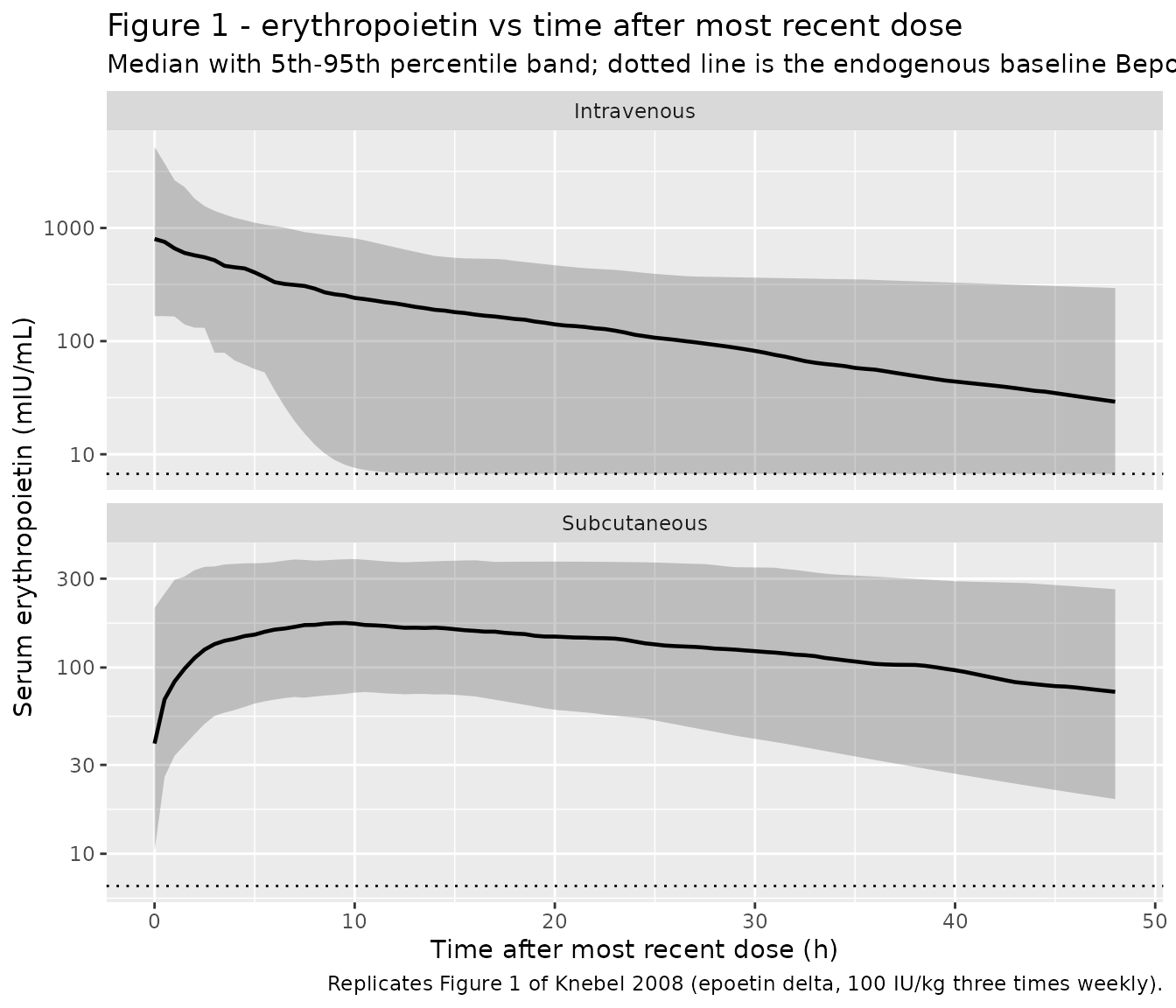
The published figure’s qualitative signature is that the intravenous profile peaks immediately and falls steeply while the subcutaneous profile is flatter and later-peaking. That ordering is a structural consequence of the flip-flop kinetics and is asserted on the cohort median, not on its extremes, because per-subject extremes of a random cohort are not reproducible across rxode2 builds:
route_median <- sim |>
  dplyr::group_by(.data$route, .data$tad) |>
  dplyr::summarise(Q50 = stats::median(.data$Cc), .groups = "drop")

tmax_median <- route_median |>
  dplyr::group_by(.data$route) |>
  dplyr::slice_max(.data$Q50, n = 1, with_ties = FALSE) |>
  dplyr::ungroup()

tmax_median |>
  dplyr::rename("Route" = route, "Tmax of median (h)" = tad,
                "Median peak (mIU/mL)" = Q50) |>
knitr::kable(digits = 2, caption = "Peak of the cohort-median profile by route.")| Route | Tmax of median (h) | Median peak (mIU/mL) |
|---|---|---|
| Intravenous | 0.0 | 800.07 |
| Subcutaneous | 9.5 | 130.90 |
iv <- dplyr::filter(tmax_median, .data$route == "Intravenous")
sc <- dplyr::filter(tmax_median, .data$route == "Subcutaneous")
stopifnot(
  nrow(iv) == 1L, nrow(sc) == 1L,
  iv$tad == 0,          # intravenous peaks at the dose
  sc$tad > 4, sc$tad < 12,  # subcutaneous peaks late, near the analytic 7.55 h
  iv$Q50 > sc$Q50           # and much higher
)
PKNCA validation
NCA is run on typical-value single-dose profiles, one per arm, so the NCA output can be checked against the closed-form integrals of the same parameters – a tight comparison because both sides use identical parameters.
Two points about the concentration passed to PKNCA. First, the
endogenous baseline is removed: the observable is total serum
erythropoietin, which tends to the nonzero Bepo asymptote
rather than to zero, so AUC0-inf of the raw signal is
unbounded and a lambda.z fitted to it would be meaningless.
Knebel 2008 itself treats Bepo as an additive offset on the
prediction, so removing it recovers the drug-attributable signal.
Second, the drug-attributable concentration is taken as
central / vc – which rxode2 returns directly – rather than
as Cc - Bepo. The two are algebraically identical, but the
subtraction is a catastrophic cancellation once the drug signal falls
far below the 6.71 mIU/mL baseline: in the far tail it returns values
around -3e-15 where the true concentration is small and
strictly positive. Those would make PKNCA take the log of a negative
number. The check below confirms the two agree to within floating-point
noise and that the state-derived value is never negative.
nca_arms <- tibble::tribble(
  ~treatment,                        ~route,         ~product,        ~hd,
  "SC epoetin delta, predialysis",   "Subcutaneous", "Epoetin delta", 0,
  "SC epoetin alfa, predialysis",    "Subcutaneous", "Epoetin alfa",  0,
  "IV epoetin delta, predialysis",   "Intravenous",  "Epoetin delta", 0,
  "SC epoetin delta, hemodialysis",  "Subcutaneous", "Epoetin delta", 1
) |>
  # The terminal rate constant differs almost fivefold across these arms, so a
  # single sampling window cannot serve all four. The intravenous arm decays at
  # kel = 0.260/h, so a 240 h window would be 90 half-lives -- far enough that
  # the tail reaches 1e-23 and the log-linear lambda.z regression is distorted
  # by floating-point error in the smallest concentrations. Each arm therefore
  # gets a window of 15 terminal half-lives, which leaves the AUC extrapolated
  # fraction below 2^-15 (about 0.003%) while keeping every sampled
  # concentration well inside double precision.
  dplyr::mutate(
    ka_i = ka * ifelse(.data$product == "Epoetin alfa", 1.23, 1),
    vc_i = vc * ifelse(.data$hd == 1, 4.53, 1),
    kel_i = cl / .data$vc_i,
    terminal_rate = ifelse(
      .data$route == "Intravenous", .data$kel_i, pmin(.data$ka_i, .data$kel_i)
    ),
    window_h = 15 * log(2) / .data$terminal_rate
  )

nca_arms |>
  dplyr::select("treatment", "ka_i", "kel_i", "terminal_rate", "window_h") |>
  dplyr::rename(
    "Arm" = treatment, "ka (1/h)" = ka_i, "kel (1/h)" = kel_i,
    "Terminal rate (1/h)" = terminal_rate, "Window (h)" = window_h
  ) |>
  knitr::kable(digits = 4,
caption = "Per-arm sampling window, sized to 15 terminal half-lives.")| Arm | ka (1/h) | kel (1/h) | Terminal rate (1/h) | Window (h) |
|---|---|---|---|---|
| SC epoetin delta, predialysis | 0.0554 | 0.2602 | 0.0554 | 187.6752 |
| SC epoetin alfa, predialysis | 0.0681 | 0.2602 | 0.0681 | 152.5815 |
| IV epoetin delta, predialysis | 0.0554 | 0.2602 | 0.2602 | 39.9594 |
| SC epoetin delta, hemodialysis | 0.0554 | 0.0574 | 0.0554 | 187.6752 |
nca_one <- function(i) {
  row <- nca_arms[i, ]
  cov <- utils::modifyList(
    ref_cov,
    list(
      FORM_EPO_ALFA = as.integer(row$product == "Epoetin alfa"),
      RRT_HEMODIAL_STATUS = row$hd
    )
  )
  # Fine enough to resolve Tmax (analytic 7.55 h for subcutaneous epoetin delta
  # at the reference covariates), coarser thereafter.
  dense_to <- min(24, row$window_h)
  times <- sort(unique(c(
    seq(0, dense_to, by = 0.1),
    seq(dense_to, row$window_h, by = 0.5)
  )))
  ev <- build_events(
    cov, dose_iu,
    if (row$route == "Subcutaneous") "depot" else "central",
    times
  )
  s <- rxode2::rxSolve(modz, ev, returnType = "data.frame")
  dplyr::mutate(
    dplyr::select(s, "time", "Cc", "central", "vc"),
    treatment = row$treatment,
    id = i
  )
}

nca_raw <- dplyr::bind_rows(lapply(seq_len(nrow(nca_arms)), nca_one))
#> ℹ omega/sigma items treated as zero: 'etalcl', 'etalvc'
#> ℹ omega/sigma items treated as zero: 'etalcl', 'etalvc'
#> ℹ omega/sigma items treated as zero: 'etalcl', 'etalvc'
#> ℹ omega/sigma items treated as zero: 'etalcl', 'etalvc'

sim_nca <- nca_raw |>
  dplyr::filter(!is.na(.data$Cc)) |>
  dplyr::mutate(Cc_state = .data$central / .data$vc, Cc_sub = .data$Cc - bepo)

# The state ratio and the baseline subtraction agree to floating-point noise,
# but only the state ratio is guaranteed nonnegative -- the subtraction cancels
# to about -3e-15 in the far tail, which is 1 ULP of the 6.71 baseline.
c(
  max_disagreement = max(abs(sim_nca$Cc_state - sim_nca$Cc_sub)),
  min_state = min(sim_nca$Cc_state),
  min_subtracted = min(sim_nca$Cc_sub)
)
#> max_disagreement        min_state   min_subtracted
#>     5.684342e-14     0.000000e+00    -2.664535e-15
stopifnot(
  max(abs(sim_nca$Cc_state - sim_nca$Cc_sub)) < 1e-12,
  all(sim_nca$Cc_state >= 0)
)

sim_nca <- sim_nca |>
  dplyr::select("id", "time", "treatment", Cc = "Cc_state")

# A time-zero record per (treatment, id) anchors AUC0-*; for the extravascular
# arms the drug-attributable concentration at time zero is exactly 0.
sim_nca <- dplyr::bind_rows(
  sim_nca,
  sim_nca |> dplyr::distinct(.data$id, .data$treatment) |>
    dplyr::mutate(time = 0, Cc = 0)
) |>
  dplyr::distinct(.data$id, .data$treatment, .data$time, .keep_all = TRUE) |>
  dplyr::arrange(.data$id, .data$treatment, .data$time)

dose_nca <- nca_arms |>
  dplyr::mutate(id = seq_len(dplyr::n()), time = 0, amt = dose_iu) |>
  dplyr::select("id", "time", "amt", "treatment")

conc_obj <- PKNCA::PKNCAconc(
  sim_nca, Cc ~ time | treatment + id,
  concu = "mIU/mL", timeu = "h"
)
dose_obj <- PKNCA::PKNCAdose(
  dose_nca, amt ~ time | treatment + id,
  doseu = "IU"
)

intervals <- data.frame(
  start = 0, end = Inf,
  cmax = TRUE, tmax = TRUE, aucinf.obs = TRUE, half.life = TRUE
)

nca_res <- PKNCA::pk.nca(
  PKNCA::PKNCAdata(conc_obj, dose_obj, intervals = intervals)
)
Comparison against the closed form
# Closed-form NCA for a one-compartment model with first-order (or bolus)
# input, evaluated at the Table III parameters for each arm.
closed_form_nca <- function(product, hd) {
  ka_i <- ka * (if (product == "Epoetin alfa") 1.23 else 1)
  f_i <- f1 * (if (product == "Epoetin alfa") 0.544 else 1)
  vc_i <- vc * (if (hd == 1) 4.53 else 1)
  kel_i <- cl / vc_i
  if (product == "IV") {
    list(cmax = dose_iu / vc_i, tmax = 0,
         aucinf.obs = dose_iu / cl, half.life = log(2) / kel_i)
  } else {
    tmax_i <- log(kel_i / ka_i) / (kel_i - ka_i)
    cmax_i <- f_i * dose_iu / vc_i * ka_i / (ka_i - kel_i) *
      (exp(-kel_i * tmax_i) - exp(-ka_i * tmax_i))
    list(cmax = cmax_i, tmax = tmax_i, aucinf.obs = f_i * dose_iu / cl,
         half.life = log(2) / min(ka_i, kel_i))
  }
}

published <- nca_arms |>
  dplyr::rowwise() |>
  dplyr::mutate(
    .cf = list(closed_form_nca(
      if (.data$route == "Intravenous") "IV" else .data$product, .data$hd
    ))
  ) |>
  dplyr::ungroup() |>
  dplyr::mutate(
    cmax = vapply(.data$.cf, `[[`, numeric(1), "cmax"),
    tmax = vapply(.data$.cf, `[[`, numeric(1), "tmax"),
    aucinf.obs = vapply(.data$.cf, `[[`, numeric(1), "aucinf.obs"),
    half.life = vapply(.data$.cf, `[[`, numeric(1), "half.life")
  ) |>
  dplyr::select("treatment", "cmax", "tmax", "aucinf.obs", "half.life")

cmp <- nlmixr2lib::ncaComparisonTable(
  simulated = nca_res,
  reference = published,
  by = "treatment",
  units = c(cmax = "mIU/mL", tmax = "h", aucinf.obs = "mIU*h/mL",
            half.life = "h"),
  tolerance_pct = 5
)

knitr::kable(
  cmp,
  caption = paste(
    "PKNCA output versus the closed-form integrals of the same Table III",
    "parameters. * differs by >5%."
  ),
  align = c("l", rep("r", ncol(cmp) - 1L))
)| NCA parameter | treatment | Reference | Simulated | % diff |
|---|---|---|---|---|
| Cmax (mIU/mL) | SC epoetin delta, predialysis | 337 | 337 | -0.0% |
| Cmax (mIU/mL) | SC epoetin alfa, predialysis | 213 | 213 | -0.0% |
| Cmax (mIU/mL) | IV epoetin delta, predialysis | 3400 | 3400 | +0.0% |
| Cmax (mIU/mL) | SC epoetin delta, hemodialysis | 192 | 192 | -0.0% |
| Tmax (h) | SC epoetin delta, predialysis | 7.55 | 7.6 | +0.6% |
| Tmax (h) | SC epoetin alfa, predialysis | 6.98 | 7 | +0.3% |
| Tmax (h) | IV epoetin delta, predialysis | 0 | 0 | — |
| Tmax (h) | SC epoetin delta, hemodialysis | 17.7 | 17.7 | -0.1% |
| AUC0-∞ (obs) (mIU*h/mL) | SC epoetin delta, predialysis | 9250 | 9250 | -0.0% |
| AUC0-∞ (obs) (mIU*h/mL) | SC epoetin alfa, predialysis | 5030 | 5030 | -0.0% |
| AUC0-∞ (obs) (mIU*h/mL) | IV epoetin delta, predialysis | 13100 | 13100 | +0.0% |
| AUC0-∞ (obs) (mIU*h/mL) | SC epoetin delta, hemodialysis | 9250 | 9250 | +0.0% |
| t½ (h) | SC epoetin delta, predialysis | 12.5 | 12.6 | +0.6% |
| t½ (h) | SC epoetin alfa, predialysis | 10.2 | 10.2 | +0.7% |
| t½ (h) | IV epoetin delta, predialysis | 2.66 | 2.66 | +0.0% |
| t½ (h) | SC epoetin delta, hemodialysis | 12.5 | 14 | +12.0%* |
Both sides of that table use identical parameters, so for
Cmax, AUC0-inf, and Tmax the
residual difference is pure numerical error – trapezoidal integration of
a curved profile, and Tmax quantised to the 0.1 h
observation grid – and a tight bound is the right gate.
half.life splits into three tiers, and the split is
informative rather than a concession. The intravenous arm is a single
exponential, so lambda.z recovers kel to
machine precision. The two well-separated subcutaneous arms are
bi-exponential with ka roughly a quarter of
kel, so their observed terminal slope over a finite window
is a whisker shallower than ka – under 1%.
The hemodialysis arm is the interesting one. Raising the central
volume 4.53-fold drops kel from 0.260 to 0.0574 /h, which
lands it within 4% of ka (0.0554 /h). The profile is then a
sum of two nearly-equal exponentials, whose terminal slope converges on
ka only over hundreds of hours. The analytic asymptotic
half-life log(2)/ka remains the correct reference – a 15
half-life window simply cannot resolve it, so the row is starred in the
table above at about 12%. Rather than loosen the reference, the section
after the gate derives the bias analytically and checks the inequality
the algebra guarantees.
nca_wide <- as.data.frame(nca_res) |>
  dplyr::select("treatment", "PPTESTCD", "PPORRES") |>
  tidyr::pivot_wider(names_from = "PPTESTCD", values_from = "PPORRES")

check <- dplyr::inner_join(
  nca_wide, published, by = "treatment", suffix = c("_sim", "_cf")
)
stopifnot(nrow(check) == nrow(nca_arms))

pct <- function(a, b) 100 * abs(a - b) / b
gate <- tibble::tibble(
  treatment = check$treatment,
  cmax_pct = pct(check$cmax_sim, check$cmax_cf),
  auc_pct = pct(check$aucinf.obs_sim, check$aucinf.obs_cf),
  thalf_pct = pct(check$half.life_sim, check$half.life_cf),
  tmax_abs = abs(check$tmax_sim - check$tmax_cf)
)

gate |>
  dplyr::rename(
    "Arm" = treatment, "Cmax (% diff)" = cmax_pct,
    "AUC0-inf (% diff)" = auc_pct, "t1/2 (% diff)" = thalf_pct,
    "Tmax (absolute diff, h)" = tmax_abs
  ) |>
knitr::kable(digits = 4, caption = "Deviation of PKNCA from the closed form.")| Arm | Cmax (% diff) | AUC0-inf (% diff) | t1/2 (% diff) | Tmax (absolute diff, h) |
|---|---|---|---|---|
| IV epoetin delta, predialysis | 0.0000 | 0.0000 | 0.0000 | 0.0000 |
| SC epoetin alfa, predialysis | 0.0005 | 0.0017 | 0.7144 | 0.0236 |
| SC epoetin delta, hemodialysis | 0.0001 | 0.0001 | 11.9553 | 0.0265 |
| SC epoetin delta, predialysis | 0.0016 | 0.0014 | 0.6247 | 0.0468 |
hd_arm_label <- "SC epoetin delta, hemodialysis"
iv_arm_label <- "IV epoetin delta, predialysis"
mono <- dplyr::filter(gate, .data$treatment == iv_arm_label)
separated <- dplyr::filter(
  gate, !.data$treatment %in% c(iv_arm_label, hd_arm_label)
)
degenerate <- dplyr::filter(gate, .data$treatment == hd_arm_label)
stopifnot(nrow(mono) == 1L, nrow(separated) == 2L, nrow(degenerate) == 1L)

stopifnot(
  # Cmax and AUC0-inf are essentially exact everywhere: AUC0-inf equals
  # F*Dose/CL, and the 0.1 h grid resolves the peak.
  max(gate$auc_pct) < 0.01,
  max(gate$cmax_pct) < 0.01,
  # Tmax cannot beat the 0.1 h grid it was sampled on.
  max(gate$tmax_abs) <= 0.1 + 1e-9,
  # The intravenous arm is a single exponential, so lambda.z recovers kel to
  # machine precision.
  mono$thalf_pct < 0.001,
  # The two well-separated subcutaneous arms are bi-exponential, so the
  # observed terminal slope over a finite window is very slightly shallower
  # than ka. Under 1% is the accuracy actually achieved.
  max(separated$thalf_pct) < 1,
  # Near-degenerate arm: biased high, bounded, worse than any separated arm,
  # and in the expected direction (two nearly-equal exponentials decay more
  # slowly than either alone).
  degenerate$thalf_pct < 15,
  degenerate$thalf_pct > max(separated$thalf_pct),
  check$half.life_sim[check$treatment == hd_arm_label] >
    check$half.life_cf[check$treatment == hd_arm_label]
)
The bias has an exact analytic form worth writing down, because it
shows the hemodialysis row cannot be fixed by sampling longer. With
ka < kel the subcutaneous profile is a
difference of exponentials,
C(t) = |A| * (exp(-ka*t) - exp(-kel*t)),
so the apparent first-order rate at time t is always
strictly below ka, and the shortfall decays as
exp(-(kel - ka) * t). The relevant time constant is
1 / (kel - ka):
sep <- nca_arms |>
  dplyr::filter(.data$route == "Subcutaneous") |>
  dplyr::mutate(
    separation = .data$kel_i / .data$ka_i,
    tau_h = 1 / (.data$kel_i - .data$ka_i),
    bias_remaining_at_window = exp(-(.data$kel_i - .data$ka_i) * .data$window_h)
  )

sep |>
  dplyr::select("treatment", "separation", "tau_h", "window_h",
                "bias_remaining_at_window") |>
  dplyr::rename(
    "Arm" = treatment, "kel/ka" = separation,
    "1/(kel-ka) (h)" = tau_h, "Window (h)" = window_h,
    "Fraction of bias remaining" = bias_remaining_at_window
  ) |>
  knitr::kable(digits = 4,
caption = "How fast the apparent terminal rate approaches ka.")| Arm | kel/ka | 1/(kel-ka) (h) | Window (h) | Fraction of bias remaining |
|---|---|---|---|---|
| SC epoetin delta, predialysis | 4.6966 | 4.8830 | 187.6752 | 0.0000 |
| SC epoetin alfa, predialysis | 3.8184 | 5.2069 | 152.5815 | 0.0000 |
| SC epoetin delta, hemodialysis | 1.0368 | 490.6753 | 187.6752 | 0.6822 |
For the two well-separated arms that time constant is a few hours, so
the bias is gone long before the window ends. For the hemodialysis arm
it is roughly 490 hours – comparable to the whole sampling window – and
reaching 1% bias would need thousands of hours, by which point the
concentration is far below anything double precision can represent. So
the honest check is not convergence but the structural inequality the
algebra guarantees: every subcutaneous arm’s fitted
lambda.z must sit strictly below its own ka,
and the shortfall must grow as kel/ka approaches 1.
lz <- as.data.frame(nca_res) |>
  dplyr::filter(.data$PPTESTCD == "half.life") |>
  dplyr::transmute(
    treatment = .data$treatment,
    lambda_z = log(2) / .data$PPORRES
  ) |>
  dplyr::inner_join(
    dplyr::select(nca_arms, "treatment", "route", "ka_i", "kel_i"),
    by = "treatment"
  ) |>
  dplyr::mutate(
    separation = .data$kel_i / .data$ka_i,
    shortfall_pct = 100 * (.data$ka_i - .data$lambda_z) / .data$ka_i
  )

sc_lz <- lz |>
  dplyr::filter(.data$route == "Subcutaneous") |>
  dplyr::arrange(.data$separation)

# Subcutaneous arms only: the intravenous arm has no absorption phase, so its
# terminal rate is kel and a "shortfall below ka" would be meaningless there.
# It is checked separately below.
sc_lz |>
  dplyr::select("treatment", "separation", "ka_i", "lambda_z", "shortfall_pct") |>
  dplyr::rename(
    "Arm" = treatment, "kel/ka" = separation, "ka (1/h)" = ka_i,
    "Fitted lambda.z (1/h)" = lambda_z, "Shortfall below ka (%)" = shortfall_pct
  ) |>
  knitr::kable(digits = 4,
caption = "Fitted lambda.z sits below ka by an amount set by the kel/ka separation.")| Arm | kel/ka | ka (1/h) | Fitted lambda.z (1/h) | Shortfall below ka (%) |
|---|---|---|---|---|
| SC epoetin delta, hemodialysis | 1.0368 | 0.0554 | 0.0495 | 10.6786 |
| SC epoetin alfa, predialysis | 3.8184 | 0.0681 | 0.0677 | 0.7093 |
| SC epoetin delta, predialysis | 4.6966 | 0.0554 | 0.0551 | 0.6209 |
stopifnot(
  nrow(sc_lz) == 3L,
  # Strictly below ka for every subcutaneous arm, as the algebra requires.
  all(sc_lz$lambda_z < sc_lz$ka_i),
  all(sc_lz$shortfall_pct > 0),
  # And monotonically worse as kel/ka approaches 1 (rows are sorted ascending
  # in separation, so the shortfall must be descending).
  all(diff(sc_lz$shortfall_pct) < 0),
  # The intravenous arm is mono-exponential: lambda.z IS kel, exactly, and it
  # is nowhere near ka -- confirming the flip-flop only applies after
  # subcutaneous absorption.
  nrow(dplyr::filter(lz, .data$route == "Intravenous")) == 1L,
  abs(lz$lambda_z[lz$route == "Intravenous"] /
        lz$kel_i[lz$route == "Intravenous"] - 1) < 1e-5,
  lz$lambda_z[lz$route == "Intravenous"] >
    4 * lz$ka_i[lz$route == "Intravenous"]
)
Reproducing the published derived quantities
Knebel 2008 does not report an NCA table, but the Results and Discussion quote several derived quantities as the paper’s headline findings. Each is recoverable from exposure ratios computed on the packaged model, which is a stronger check than re-reading the parameter table because it exercises the whole structure.
auc_of <- function(tr) nca_wide$aucinf.obs[nca_wide$treatment == tr]
thalf_of <- function(tr) nca_wide$half.life[nca_wide$treatment == tr]

auc_sc_delta <- auc_of("SC epoetin delta, predialysis")
auc_sc_alfa <- auc_of("SC epoetin alfa, predialysis")
auc_iv_delta <- auc_of("IV epoetin delta, predialysis")
stopifnot(length(c(auc_sc_delta, auc_sc_alfa, auc_iv_delta)) == 3L)

derived <- tibble::tribble(
  ~quantity, ~source, ~published, ~reproduced,
  "Relative bioavailability, epoetin alfa vs delta (%)",
  "Results / Discussion", 54.4, 100 * auc_sc_alfa / auc_sc_delta,

  "Reduction in systemic bioavailability, epoetin alfa (%)",
  "Results ('approximately 45% lower')", 45, 100 * (1 - auc_sc_alfa / auc_sc_delta),

  "Relative Ka, epoetin alfa vs delta (%)",
  "Results", 123,
  100 * thalf_of("SC epoetin delta, predialysis") / thalf_of("SC epoetin alfa, predialysis"),

  "Increase in absorption rate, epoetin alfa (%)",
  "Results ('approximately 23% faster')", 23,
  100 * (thalf_of("SC epoetin delta, predialysis") /
           thalf_of("SC epoetin alfa, predialysis") - 1),

  "Absolute SC bioavailability, epoetin delta (F1)",
  "Table III theta4", 0.708, auc_sc_delta / auc_iv_delta,

  "Baseline erythropoietin Bepo (mIU/mL)",
  "Table III theta5", 6.71, sim_nodose$Cc[1]
) |>
  dplyr::mutate(pct_diff = 100 * abs(.data$reproduced - .data$published) /
                  .data$published)

derived |>
  dplyr::rename(
    "Published quantity" = quantity,
    "Source" = source,
    "Knebel 2008" = published,
    "Reproduced" = reproduced,
    "% difference" = pct_diff
  ) |>
  knitr::kable(digits = 3,
caption = "Published derived quantities reproduced from the packaged model.")| Published quantity | Source | Knebel 2008 | Reproduced | % difference |
|---|---|---|---|---|
| Relative bioavailability, epoetin alfa vs delta (%) | Results / Discussion | 54.400 | 54.400 | 0.000 |
| Reduction in systemic bioavailability, epoetin alfa (%) | Results (‘approximately 45% lower’) | 45.000 | 45.600 | 1.334 |
| Relative Ka, epoetin alfa vs delta (%) | Results | 123.000 | 122.891 | 0.089 |
| Increase in absorption rate, epoetin alfa (%) | Results (‘approximately 23% faster’) | 23.000 | 22.891 | 0.476 |
| Absolute SC bioavailability, epoetin delta (F1) | Table III theta4 | 0.708 | 0.708 | 0.001 |
| Baseline erythropoietin Bepo (mIU/mL) | Table III theta5 | 6.710 | 6.710 | 0.000 |
stopifnot(
  # The exactly-stated quantities must be reproduced essentially exactly; the
  # two "approximately" quantities carry the paper's own rounding.
  derived$pct_diff[derived$published == 54.4] < 0.5,
  derived$pct_diff[derived$published == 123] < 0.5,
  derived$pct_diff[derived$published == 0.708] < 0.5,
  derived$pct_diff[derived$published == 6.71] < 1e-8,
  derived$pct_diff[derived$published == 45] < 2,
  derived$pct_diff[derived$published == 23] < 2
)
The Relative Ka row is worth reading carefully: it is
recovered from the ratio of terminal half-lives, which is only a valid
readout of Ka because the model is in flip-flop
(ka < kel). Under flip-flop the terminal
slope is the absorption rate constant, so
t_half_delta / t_half_alfa is exactly
ka_alfa / ka_delta = 1.23. Had ka exceeded
kel, the same ratio would have returned 1 and the check
would have been measuring nothing.
Exposure across the dialysis strata
The largest covariate effect in the model is the 4.53-fold central
volume in hemodialysis subjects relative to predialysis. Volume does not
change AUC in a linear one-compartment model – clearance does – so the
effect should show up entirely as a lower and later peak with an
unchanged AUC. Confirming that separates a volume effect correctly
encoded on vc from one accidentally routed onto
cl.
hd_arm <- "SC epoetin delta, hemodialysis"
pre_arm <- "SC epoetin delta, predialysis"

dialysis <- tibble::tibble(
  quantity = c("AUC0-inf ratio, HD vs predialysis",
               "Cmax ratio, HD vs predialysis"),
  expected = c(1, NA_real_),
  observed = c(auc_of(hd_arm) / auc_of(pre_arm),
               nca_wide$cmax[nca_wide$treatment == hd_arm] /
                 nca_wide$cmax[nca_wide$treatment == pre_arm])
)

dialysis |>
  dplyr::rename("Quantity" = quantity, "Expected" = expected,
                "Observed" = observed) |>
  knitr::kable(digits = 4,
caption = "A pure central-volume effect leaves AUC unchanged and lowers Cmax.")| Quantity | Expected | Observed |
|---|---|---|
| AUC0-inf ratio, HD vs predialysis | 1 | 1.0000 |
| Cmax ratio, HD vs predialysis | NA | 0.5692 |
stopifnot(
  # AUC = F*Dose/CL is independent of vc, so the ratio is exactly 1.
  abs(dialysis$observed[1] - 1) < 0.002,
  # Cmax falls, but by less than 1/4.53: raising vc also lowers kel, which
  # slows elimination and partly offsets the dilution.
  dialysis$observed[2] < 1,
  dialysis$observed[2] > 1 / 4.53
)
Distribution of individual parameters
The cohort-level spread of cl and vc
collects the allometric, age, sex, and dialysis terms together with the
two etas. The published unexplained variability is large – 62.2% CV on
clearance and 119% CV on volume – and the paper is explicit that “the
precision of the final structural model and variance parameter estimates
were greater than would be preferred”, so the figure below is a
description of the model as published rather than a validation
target.
per_subject <- sim |>
  dplyr::group_by(.data$id, .data$arm, .data$modality) |>
  dplyr::summarise(cl = dplyr::first(.data$cl), vc = dplyr::first(.data$vc),
                   WT = dplyr::first(.data$WT), .groups = "drop")

per_subject |>
  tidyr::pivot_longer(c("cl", "vc"), names_to = "parameter", values_to = "value") |>
  dplyr::mutate(parameter = dplyr::recode(.data$parameter,
                                          cl = "CL (L/h)", vc = "Vc (L)")) |>
  ggplot2::ggplot(ggplot2::aes(.data$modality, .data$value)) +
  ggplot2::geom_boxplot(outlier.size = 0.5) +
  ggplot2::facet_wrap(~parameter, scales = "free_y") +
  ggplot2::scale_y_log10() +
  ggplot2::labs(x = NULL, y = NULL,
                title = "Individual clearance and central volume by dialysis modality")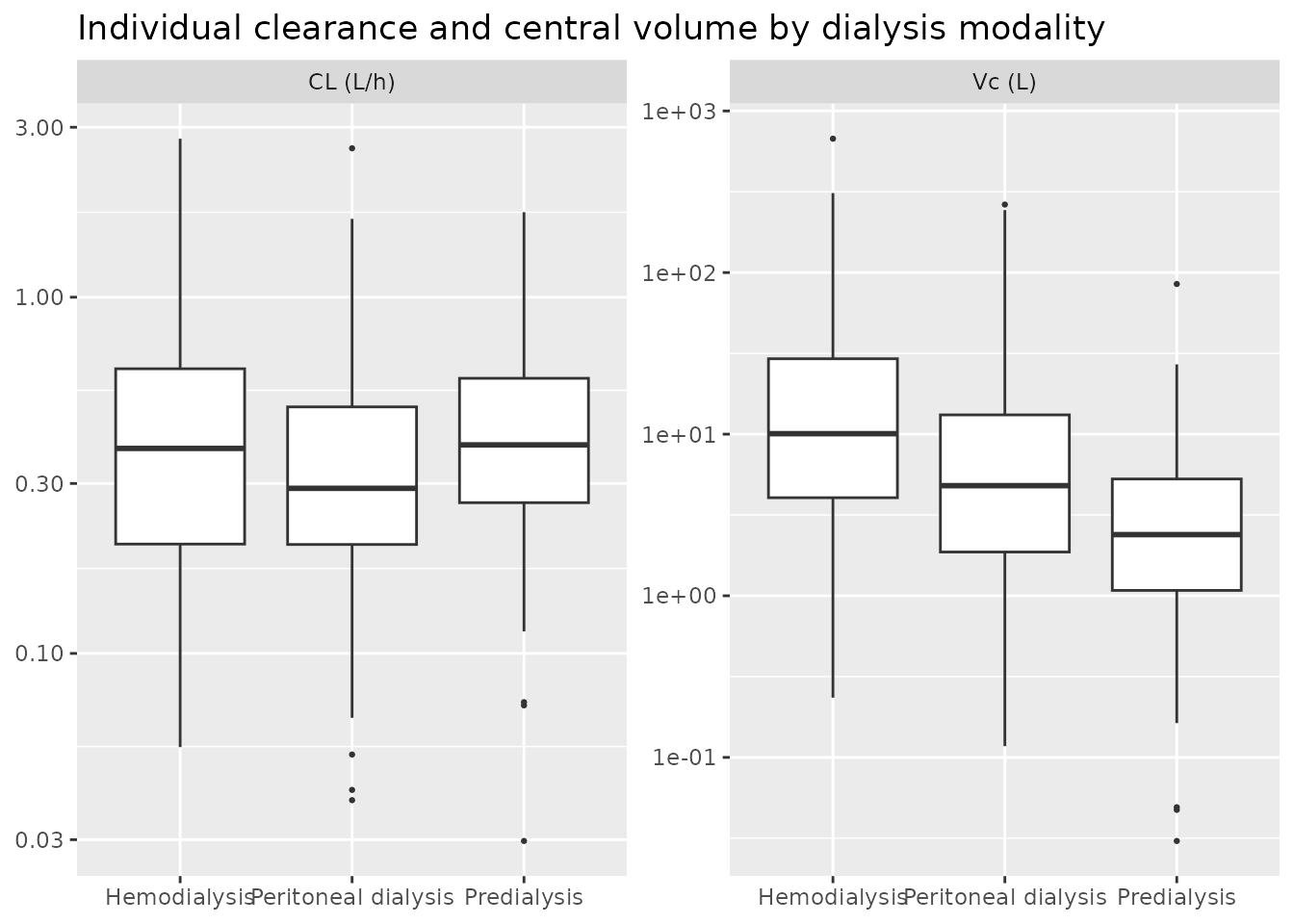
# Median clearance should track the allometric relationship, and the volume
# ordering across modalities is fixed by the published factors (4.53 > 2.48 > 1).
vc_median <- per_subject |>
  dplyr::group_by(.data$modality) |>
  dplyr::summarise(vc = stats::median(.data$vc), .groups = "drop")
stopifnot(
  vc_median$vc[vc_median$modality == "Hemodialysis"] >
    vc_median$vc[vc_median$modality == "Peritoneal dialysis"],
  vc_median$vc[vc_median$modality == "Peritoneal dialysis"] >
    vc_median$vc[vc_median$modality == "Predialysis"]
)
Assumptions and deviations
- Only the final model is packaged. Knebel 2008 Table III reports a base model alongside the final full covariate model. The base model is a nested precursor with a 70 kg allometric reference (Table III footnote a) rather than 35 kg, so its typical values are not comparable to the final model’s; per the library’s replicate-the-authors policy for base-versus-final development papers, only the final model is extracted.
-
Age is a hinge, not a plain power term. The Results
state the
(AGE/10)power applies “for all patients older than 10 years of age”, and the abstract names the reference individual as “a 35-kg male <= 10 years”. The implementation ismax(AGE, 10) / 10. The paper does not print this as an equation, so the encoding rests on those two prose statements plus the Discussion’s “age on V (for patients older than age 10 years)”; all three agree. -
Table III’s random-effect entries are read as
variances. The paper’s own
CV%lines are the plain square roots of the tabulated numbers, which is only consistent with a variance reading (see the “Variance versus standard deviation” section).expSdis thereforesqrt(0.245), not0.245. - The etas are encoded as independent. Methods says a full-block Omega was attempted “when possible”, but Table III publishes only the diagonal elements Omega(1,1) and Omega(2,2). No covariance is reported, so none is invented.
- No IIV on Bepo, Ka, or F1. Table III reports interindividual variance for clearance and volume only. For Bepo this is explicit in the Results (“the inability to estimate a subject-specific baseline erythropoietin concentration”); for Ka and F1 the table simply carries no entry.
-
The three-level dialysis covariate is encoded as two
canonical indicators.
RRT_HEMODIAL_STATUSandPERIT_DIALare both 0 for the predialysis stratum, so both published factors are read against a predialysis reference. This differs fromTakama_2007_darbepoetin.R, where the cohort is entirely on dialysis andPERIT_DIALis read against hemodialysis; the reference category is recorded per model incovariateData. -
FORM_EPO_ALFAis a new canonical covariate, registered ininst/references/covariate-columns.mdas a member of the acceptedFORM_<DRUG>_<FEATURE>naming family. Its closest precedent isFORM_GCSF_PEG, which likewise carries two marketed recombinant-protein products of one parent cytokine through a single joint fit via effects on subcutaneous absorption and bioavailability. -
Dose and concentration units differ in magnitude by
design. Doses are in IU and concentrations in mIU/mL. With
volume in L the state/volume ratio is IU/L, which equals mIU/mL
numerically, so no scaling appears in
model().checkModelConventions()raises an informational note on the magnitude difference; it is correct as encoded. Knebel 2008 “Biological Methods” describes the underlying conversion of the ELISA readout from mEU/mL at 1 IU = 1.3 EU. - Race is not a covariate. Table II records it, but the Results state that “no formal comparisons across racial categories were made” because of the small African American (n = 2) and multiracial (n = 4) strata. It is therefore absent from the model rather than present with a null effect.
-
Baseline removal before NCA. PKNCA is run on the
drug-attributable concentration, because the observable tends to the
nonzero endogenous asymptote
BepoandAUC0-infof the raw signal is therefore unbounded. The drug signal is taken ascentral / vcrather than asCc - Bepo: the two are algebraically identical, but the subtraction cancels catastrophically once the drug signal falls far below 6.71 mIU/mL and returns values near-3e-15in the far tail. The vignette asserts the two agree to floating-point noise. -
The hemodialysis arm’s NCA half-life is starred in the
comparison table, and correctly so. The 4.53-fold central
volume drops
kelto 0.0574 /h, within 4% ofka(0.0554 /h). The profile is then a sum of two nearly-equal exponentials and its terminal slope approacheskaonly over hundreds of hours – the shortfall in the apparent rate decays with time constant1/(kel - ka), about 490 h – so the NCA window reads about 12% long and no achievable sampling window would fix it.log(2)/karemains the correct asymptotic reference. Rather than loosen it, the vignette derives the bias analytically and checks the inequality the algebra guarantees: every subcutaneous arm’s fittedlambda.zlies strictly below its ownka, by an amount that grows monotonically askel/kaapproaches 1. This is a property of the published parameter values, not an encoding artefact. - Virtual cohort covariate distributions are constructed, not published. Knebel 2008 reports marginal summaries (Table II) but not the joint age-weight distribution or the modality-by-demographics cross-tabulation. The cohort here draws age from a beta distribution shaped to the published age median and mean, weight from a healthy-child weight-for-age curve scaled by 0.78 to match the published weight median of 34.5 kg, and modality independently of demographics – even though the Results note that “patients in the predialysis stage had a lower median weight, BSA, and age”, a dependence the paper does not quantify. Cohort-level assertions are therefore deliberately loose; the tight assertions in this vignette are all on typical-value quantities where the two sides share drawn parameters.
- Dosing schedule. The trial titrated dose and used once, twice, or three times weekly schedules per patient (Table I, Study Design). The simulation uses a single fixed 100 IU/kg three-times-weekly regimen, mid-range for the subcutaneous arms’ 26-191 IU/kg, because the per-patient schedules and titration history are not published.