Nicotine and cotinine PBPK in non-pregnant women (Amice 2021)

Model and source

• Citation: Amice B, Ho H, Zhang E, Bullen C. (2021). Physiologically Based Pharmacokinetic Modelling for Nicotine and Cotinine Clearance in Pregnant Women. Front Pharmacol 12:688597. doi:10.3389/fphar.2021.688597. PMCID PMC8329445. Equations from Supplementary DataSheet 1 (Eqs 1-22); physiological and drug parameters from Supplementary DataSheet 2 (Tables S.1 and S.3) and main-text Table 1. Framework inherited from Robinson DE, Balter NJ, Schwartz SL (1992) J Pharmacokinet Biopharm 20:591-609, doi:10.1007/BF01064421.

• Description: PBPK (whole-body, in-house MATLAB). Nicotine and cotinine disposition in a non-pregnant adult woman after intravenous dosing (Amice 2021, ‘Baseline PBPK Model’). Nine flow-limited nicotine compartments (arterial and venous blood, lung, brain, liver, kidney, rapidly perfused, slowly perfused and fat) and nine matching cotinine compartments, coupled in the liver where 80 percent of hepatic nicotine clearance forms cotinine; renal and hepatic clearances act on the unbound tissue-outflow concentration, with urine and metabolised-mass accumulators for each analyte. Deterministic typical-value model: the source reports no between-subject variability and no residual-error model. The paper’s pregnancy model (mammary, uterus, placenta and a four-compartment fetus) is NOT implemented, because its placental transfer equations contradict the supplement tables and several of its parameters are unpublished; see the vignette Errata.

• Article: https://doi.org/10.3389/fphar.2021.688597 (open access, PMC8329445)

• Supplementary material (DataSheet 1: equations; DataSheet 2: Tables S.1-S.3): https://www.frontiersin.org/articles/10.3389/fphar.2021.688597/full#supplementary-material

Amice 2021 is a short research report on a whole-body PBPK model for nicotine and its main metabolite cotinine, written in MATLAB and solved with ode45. The paper presents two models: a baseline adult model for a non-pregnant woman, and a pregnancy (p-PBPK) model that adds mammary, uterus, placenta and a fetus. Only the baseline non-pregnant model is packaged here. The pregnancy model cannot be reproduced from the published material; the reasons are listed under Assumptions and deviations.

Population

The model is a physiological simulation, not a fit to individual data. The baseline woman weighs 70 kg (Results, “Baseline PBPK Model”, following the adult configuration of Robinson 1992). Her hepatic and renal clearances are the Dempsey 2002 values for women (Table 1, column 2). Her organ volumes and blood flows are the adult fractions of Supplementary Table S.1, and her drug-specific partition coefficients, unbound fractions and blood:plasma ratios come from Supplementary Table S.3.

The authors checked the baseline model against two published intravenous studies in non-smokers: plasma nicotine and cotinine in six subjects given nicotine at 10 ug/min for 60 min (Curvall 1990), and plasma cotinine in four subjects given cotinine at 0.67 mg/min for 30 min (De Schepper 1987).

The same information is available programmatically:

str(readModelDb("Amice_2021_nicotine_pbpk")()$population)
#> List of 8
#>  $ species       : chr "human"
#>  $ n_subjects    : int NA
#>  $ age_range     : chr "adult"
#>  $ weight_median : chr "70 kg reference adult woman (Amice 2021 Results 'Baseline PBPK Model', after Robinson 1992)"
#>  $ sex_female_pct: num 100
#>  $ disease_state : chr "healthy non-pregnant adult women (non-smokers in the validation datasets)"
#>  $ dose_range    : chr "intravenous nicotine 10 ug/min for 60 min (Curvall 1990 regimen); intravenous cotinine 0.67 mg/min for 30 min ("| __truncated__
#>  $ notes         : chr "A PBPK model, not fitted to individual-level data. The hepatic and renal clearances for women are the Dempsey 2"| __truncated__

Source trace

Each ini() value carries an in-file comment naming its source. The table collects them. “DS1” is Supplementary DataSheet 1 (the equations) and “DS2” is Supplementary DataSheet 2 (Tables S.1-S.3).

Equation / parameter	Value	Source location
Arterial blood, d/dt(a_arterial)	n/a	DS1 Eq 1 (nicotine), Eq 12 (cotinine)
Fat, slowly perfused, rapidly perfused, brain	n/a	DS1 Eqs 2-5 and 13-16
Kidney, with renal clearance fu * CL_renal * C_K / K_K	n/a	DS1 Eqs 8 and 19
Liver, with hepatic clearance fu * CL_hep * C_Li / K_Li	n/a	DS1 Eqs 9 and 20
Cotinine formation 0.8 * fuN * CLN_Li * CN_Li / KN_Li	n/a	DS1 Eq 20
Lung	n/a	DS1 Eqs 10 and 21
Venous blood, with the intravenous dose input	n/a	DS1 Eqs 11 and 22
qcc (cardiac output = qcc * WT^0.75)	15.126 L/h/kg^0.75	DS2 Table S.1, FCO
fvol_arterial, fvol_venous	0.02, 0.0571	DS2 Table S.1
fvol_fat, fvol_slowly_perfused, fvol_rapidly_perfused	0.187, 0.536, 0.032	DS2 Table S.1
fvol_brain, fvol_kidney, fvol_liver, fvol_lung	0.021, 0.004, 0.026, 0.008	DS2 Table S.1
fq_fat, fq_slowly_perfused, fq_rapidly_perfused	0.052, 0.188, 0.216	DS2 Table S.1
fq_brain, fq_kidney, fq_liver	0.117, 0.177, 0.25	DS2 Table S.1
lclint, lcl_renal (nicotine)	log(16.2), log(0.7) mL/min/kg	Table 1, women; DS2 Table S.3
lclint_cot, lcl_renal_cot (cotinine)	log(0.5), log(0.2) mL/min/kg	Table 1, women; DS2 Table S.3
fu, fu_cot	0.95, 0.974	DS2 Table S.3
bpr, bpr_cot	0.8, 0.88	DS2 Table S.3
fm	0.8	DS1 Eq 20; Methods (“approximately 80%”)
lkp_fat, lkp_slowly_perfused, lkp_rapidly_perfused, lkp_brain	log(1), log(2.5), log(3), log(3)	DS2 Table S.3, nicotine
lkp_kidney, lkp_liver, lkp_lung	log(15), log(9), log(2)	DS2 Table S.3, nicotine
lkp_fat_cot, lkp_slowly_perfused_cot, lkp_rapidly_perfused_cot, lkp_brain_cot	log(0.5), log(0.85), log(1.5), log(1.5)	DS2 Table S.3, cotinine
lkp_kidney_cot, lkp_liver_cot, lkp_lung_cot	log(2), log(2), log(1)	DS2 Table S.3, cotinine

Simulation scenarios

The model is deterministic, so each scenario is a single 70 kg woman. The three regimens are the ones the paper simulates for the non-pregnant woman.

mod <- readModelDb("Amice_2021_nicotine_pbpk")

# Doses go to the venous blood state of the analyte given. Observation rows
# sit on the same ODE state; rxode2 returns every algebraic output (Cc,
# Cc_cot, Cbrain, ...) at those rows.
make_events <- function(amt, rate, cmt, obs_times, id) {
  dose <- data.frame(id = id, time = 0, evid = 1, amt = amt, rate = rate, cmt = cmt)
  obs <- data.frame(id = id, time = obs_times, evid = 0, amt = 0, rate = 0, cmt = cmt)
  dplyr::bind_rows(dose, obs) |>
    dplyr::arrange(time, dplyr::desc(evid)) |>
    dplyr::mutate(WT = 70)
}

# Scenario 1 (Figure 2A): nicotine 10 ug/min for 60 min = 600 ug at 600 ug/h.
ev_nic <- make_events(600, 600, "a_venous", seq(0, 48, by = 1 / 12), id = 1L)
# Scenario 2 (Figure 2B): cotinine 0.67 mg/min for 30 min = 20100 ug at 40200 ug/h.
ev_cot <- make_events(20100, 40200, "a_venous_cot", seq(0, 24, by = 1 / 12), id = 2L)
# Scenario 3 (Figure 3A): single intravenous nicotine injection of 1 ug/kg.
ev_bolus <- make_events(70, 0, "a_venous", seq(0, 1, by = 1 / 120), id = 3L)

sim_nic <- as.data.frame(rxode2::rxSolve(mod, events = ev_nic))
sim_cot <- as.data.frame(rxode2::rxSolve(mod, events = ev_cot))
sim_bolus <- as.data.frame(rxode2::rxSolve(mod, events = ev_bolus))

Mass balance

Every nicotine state plus the metabolised-nicotine accumulator must add up to the dose. Every cotinine state plus the metabolised-cotinine accumulator must add up to fm times the metabolised nicotine. Both sides use the same solve, so the difference is pure integration error and the bound is tight.

nic_states <- c(
  "a_arterial", "a_fat", "a_slowly_perfused", "a_rapidly_perfused", "a_brain",
  "a_kidney", "a_liver", "a_lung", "a_venous", "a_urine", "a_hepatic"
)
cot_states <- paste0(setdiff(nic_states, "a_hepatic"), "_cot")
mb <- sim_nic |>
  dplyr::filter(time >= 1) |>
  dplyr::mutate(
    nic_total = rowSums(dplyr::pick(dplyr::all_of(nic_states))),
    cot_total = rowSums(dplyr::pick(dplyr::all_of(c(cot_states, "a_hepatic_cot"))))
  )
stopifnot(
  max(abs(mb$nic_total - 600)) < 1e-3,
  max(abs(mb$cot_total - 0.8 * mb$a_hepatic)) < 1e-3
)

Replicate published figures

Figure 2A: nicotine infusion, plasma nicotine and cotinine

The maintainers digitised the authors’ model curves (blue and red lines) from Figure 2A. The model output overlaid below is plasma (blood divided by the Table S.3 blood:plasma ratio).

fig2a <- tibble::tribble(
  ~time_min, ~analyte,   ~paper,
  15,        "Nicotine", 2.07,
  30,        "Nicotine", 3.40,
  45,        "Nicotine", 4.26,
  100,       "Nicotine", 2.55,
  150,       "Nicotine", 1.94,
  200,       "Nicotine", 1.60,
  250,       "Nicotine", 1.32,
  295,       "Nicotine", 1.12,
  45,        "Cotinine", 2.18,
  100,       "Cotinine", 3.95,
  200,       "Cotinine", 4.96
)

sim_fig2a <- sim_nic |>
  dplyr::filter(time <= 5) |>
  dplyr::select(time, Nicotine = Cc, Cotinine = Cc_cot) |>
  tidyr::pivot_longer(-time, names_to = "analyte", values_to = "conc")

ggplot(sim_fig2a, aes(time * 60, conc, colour = analyte)) +
  geom_line() +
  geom_point(data = fig2a, aes(time_min, paper), shape = 4, size = 2.5) +
  scale_y_log10(limits = c(0.1, 10)) +
  labs(
    x = "Time (min)", y = "Plasma concentration (ug/L)", colour = NULL,
    title = "Nicotine 10 ug/min for 60 min, 70 kg woman",
    caption = "Replicates Figure 2A of Amice 2021. Crosses: authors' model curves, digitised."
  )
#> Warning in scale_y_log10(limits = c(0.1, 10)): log-10 transformation introduced
#> infinite values.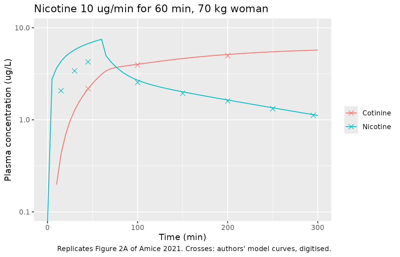

fig2a_cmp <- fig2a |>
  dplyr::mutate(
    model = mapply(
      function(t, a) {
        col <- if (a == "Nicotine") "Cc" else "Cc_cot"
        stats::approx(sim_nic$time * 60, sim_nic[[col]], xout = t)$y
      },
      time_min, analyte
    ),
    pct_diff = 100 * (model / paper - 1)
  )

fig2a_cmp |>
  dplyr::mutate(model = round(model, 2), pct_diff = round(pct_diff, 1)) |>
  dplyr::rename(
    "Time (min)" = time_min, "Analyte" = analyte,
    "Figure 2A (ug/L)" = paper, "Model (ug/L)" = model, "Difference (%)" = pct_diff
  ) |>
  knitr::kable(caption = "Model plasma concentrations against the digitised Figure 2A curves.")

Model plasma concentrations against the digitised Figure 2A curves.

Time (min)	Analyte	Figure 2A (ug/L)	Model (ug/L)	Difference (%)
15	Nicotine	2.07	4.33	109.0
30	Nicotine	3.40	5.76	69.4
45	Nicotine	4.26	6.73	57.9
100	Nicotine	2.55	2.69	5.5
150	Nicotine	1.94	2.01	3.8
200	Nicotine	1.60	1.64	2.5
250	Nicotine	1.32	1.35	2.3
295	Nicotine	1.12	1.14	1.5
45	Cotinine	2.18	2.18	-0.2
100	Cotinine	3.95	4.01	1.5
200	Cotinine	4.96	5.12	3.3

# After the infusion (100 min onwards) and for cotinine throughout, the model
# reproduces the authors' curves within digitisation error (observed range
# -0.2% to +5.5%). During the nicotine infusion it does not: see the deviations.
post <- dplyr::filter(fig2a_cmp, analyte == "Cotinine" | time_min >= 100)
stopifnot(max(abs(post$pct_diff)) < 12)

Urinary recovery at 5 h

The paper states its model’s urinary recovery 5 h after the start of the nicotine infusion: 28.8 ug unchanged nicotine and 15.3 ug cotinine (Results, “Baseline PBPK Model”). Curvall 1990 measured 22 +/- 7.2 ug and 16.1 +/- 3.8 ug.

at5 <- dplyr::filter(sim_nic, abs(time - 5) < 1e-8)
urine <- tibble::tibble(
  Analyte = c("Nicotine", "Cotinine"),
  `Amice 2021 model (ug)` = c(28.8, 15.3),
  `Curvall 1990 observed (ug)` = c("22 +/- 7.2", "16.1 +/- 3.8"),
  `This model (ug)` = round(c(at5$a_urine, at5$a_urine_cot), 1)
)
knitr::kable(urine, caption = "Cumulative urinary excretion 0-5 h after nicotine 10 ug/min for 60 min.")

Cumulative urinary excretion 0-5 h after nicotine 10 ug/min for 60 min.

Analyte	Amice 2021 model (ug)	Curvall 1990 observed (ug)	This model (ug)
Nicotine	28.8	22 +/- 7.2	28.9
Cotinine	15.3	16.1 +/- 3.8	14.6

stopifnot(
  abs(at5$a_urine / 28.8 - 1) < 0.03,
  abs(at5$a_urine_cot / 15.3 - 1) < 0.08
)

Figure 2B: cotinine infusion

Figure 2B shows the authors’ model (blue) and De Schepper 1987’s observed plasma cotinine (red), both digitised by the maintainers.

fig2b <- tibble::tribble(
  ~time, ~paper_model, ~observed,
  1,     292,          383,
  2,     260,          328,
  5,     226,          276,
  10,    175,          220,
  20,    106,          129,
  23.5,  89,           107
)

fig2b_cmp <- fig2b |>
  dplyr::mutate(
    plasma = stats::approx(sim_cot$time, sim_cot$Cc_cot, xout = time)$y,
    blood = stats::approx(sim_cot$time, sim_cot$Cblood_cot, xout = time)$y
  )

sim_cot |>
  dplyr::select(time, `Model, plasma` = Cc_cot, `Model, whole blood` = Cblood_cot) |>
  tidyr::pivot_longer(-time, names_to = "series", values_to = "conc") |>
  ggplot(aes(time, conc)) +
  geom_line(aes(linetype = series)) +
  geom_point(data = fig2b, aes(time, paper_model, colour = "Amice 2021 model"), shape = 4, size = 2.5) +
  geom_point(data = fig2b, aes(time, observed, colour = "De Schepper 1987 observed"), size = 2) +
  scale_y_log10(limits = c(10, 1000)) +
  labs(
    x = "Time (h)", y = "Cotinine (ug/L)", colour = "Digitised", linetype = NULL,
    title = "Cotinine 0.67 mg/min for 30 min, 70 kg woman",
    caption = "Replicates Figure 2B of Amice 2021."
  )
#> Warning in scale_y_log10(limits = c(10, 1000)): log-10 transformation
#> introduced infinite values.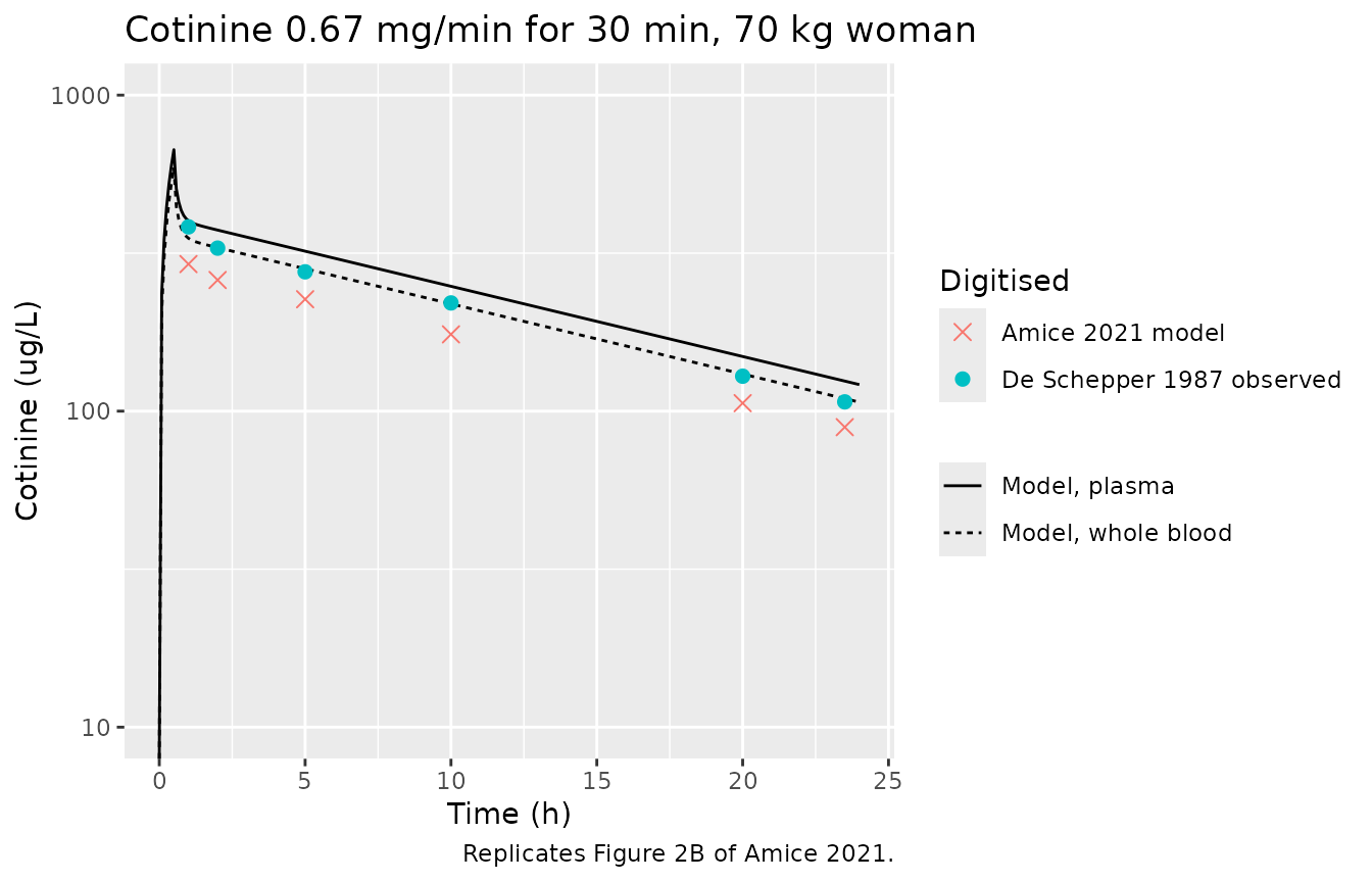

fig2b_cmp |>
  dplyr::mutate(dplyr::across(c(plasma, blood), \(x) round(x, 0))) |>
  dplyr::rename(
    "Time (h)" = time, "Figure 2B model (ug/L)" = paper_model,
    "De Schepper observed (ug/L)" = observed,
    "This model, plasma (ug/L)" = plasma, "This model, blood (ug/L)" = blood
  ) |>
  knitr::kable(caption = "Cotinine after the cotinine infusion.")

Cotinine after the cotinine infusion.

Time (h)	Figure 2B model (ug/L)	De Schepper observed (ug/L)	This model, plasma (ug/L)	This model, blood (ug/L)
1.0	292	383	400	352
2.0	260	328	374	329
5.0	226	276	321	282
10.0	175	220	248	219
20.0	106	129	149	131
23.5	89	107	124	110

# The level is offset (see the deviations); the terminal slope is not. Both
# the digitised curve and the model give a 10-20 h half-life of about 13-14 h.
hl <- function(t, c) log(2) * diff(t) / -diff(log(c))
hl_paper <- hl(fig2b$time[c(4, 5)], fig2b$paper_model[c(4, 5)])
hl_model <- hl(fig2b_cmp$time[c(4, 5)], fig2b_cmp$plasma[c(4, 5)])
c(paper = hl_paper, model = hl_model)
#>    paper    model 
#> 13.82570 13.54846
stopifnot(abs(hl_model / hl_paper - 1) < 0.15)

Figure 3A: maternal brain after a 1 ug/kg nicotine injection

Figure 3A shows maternal brain concentrations after a single 1 ug/kg intravenous nicotine injection, for the pregnant and the non-pregnant woman. The maintainers digitised all four curves. By the legend, the solid line is pregnant nicotine, the dotted line non-pregnant nicotine, the dashed line pregnant cotinine and the blue line non-pregnant cotinine.

fig3a <- tibble::tribble(
  ~time_min, ~analyte,   ~solid_or_dashed, ~dotted_or_blue,
  2.5,       "Nicotine", 4.65,             6.46,
  5,         "Nicotine", 4.32,             6.11,
  10,        "Nicotine", 3.54,             5.09,
  20,        "Nicotine", 2.24,             3.35,
  30,        "Nicotine", 1.53,             2.28,
  45,        "Nicotine", 1.04,             1.53,
  10,        "Cotinine", 0.318,            0.268,
  20,        "Cotinine", 0.484,            0.432,
  30,        "Cotinine", 0.521,            0.471,
  45,        "Cotinine", 0.531,            0.498
)

fig3a_cmp <- fig3a |>
  dplyr::mutate(
    model = mapply(
      function(t, a) {
        col <- if (a == "Nicotine") "Cbrain" else "Cbrain_cot"
        stats::approx(sim_bolus$time * 60, sim_bolus[[col]], xout = t)$y
      },
      time_min, analyte
    ),
    pct_vs_solid_or_dashed = 100 * (model / solid_or_dashed - 1),
    pct_vs_dotted_or_blue = 100 * (model / dotted_or_blue - 1)
  )

sim_bolus |>
  dplyr::select(time, Nicotine = Cbrain, Cotinine = Cbrain_cot) |>
  tidyr::pivot_longer(-time, names_to = "analyte", values_to = "conc") |>
  dplyr::filter(conc > 1e-3) |>
  ggplot(aes(time * 60, conc, colour = analyte)) +
  geom_line() +
  geom_point(data = fig3a, aes(time_min, solid_or_dashed, shape = "Solid / dashed (legend: pregnant)"), size = 2.5) +
  geom_point(data = fig3a, aes(time_min, dotted_or_blue, shape = "Dotted / blue (legend: non-pregnant)"), size = 2.5) +
  scale_shape_manual(values = c(4, 1)) +
  scale_y_log10(limits = c(1e-3, 10)) +
  labs(
    x = "Time (min)", y = "Brain concentration (ug/L)", colour = NULL, shape = "Figure 3A curve",
    title = "Single intravenous nicotine injection, 1 ug/kg, 70 kg woman",
    caption = "Replicates Figure 3A of Amice 2021. Points: digitised curves."
  )

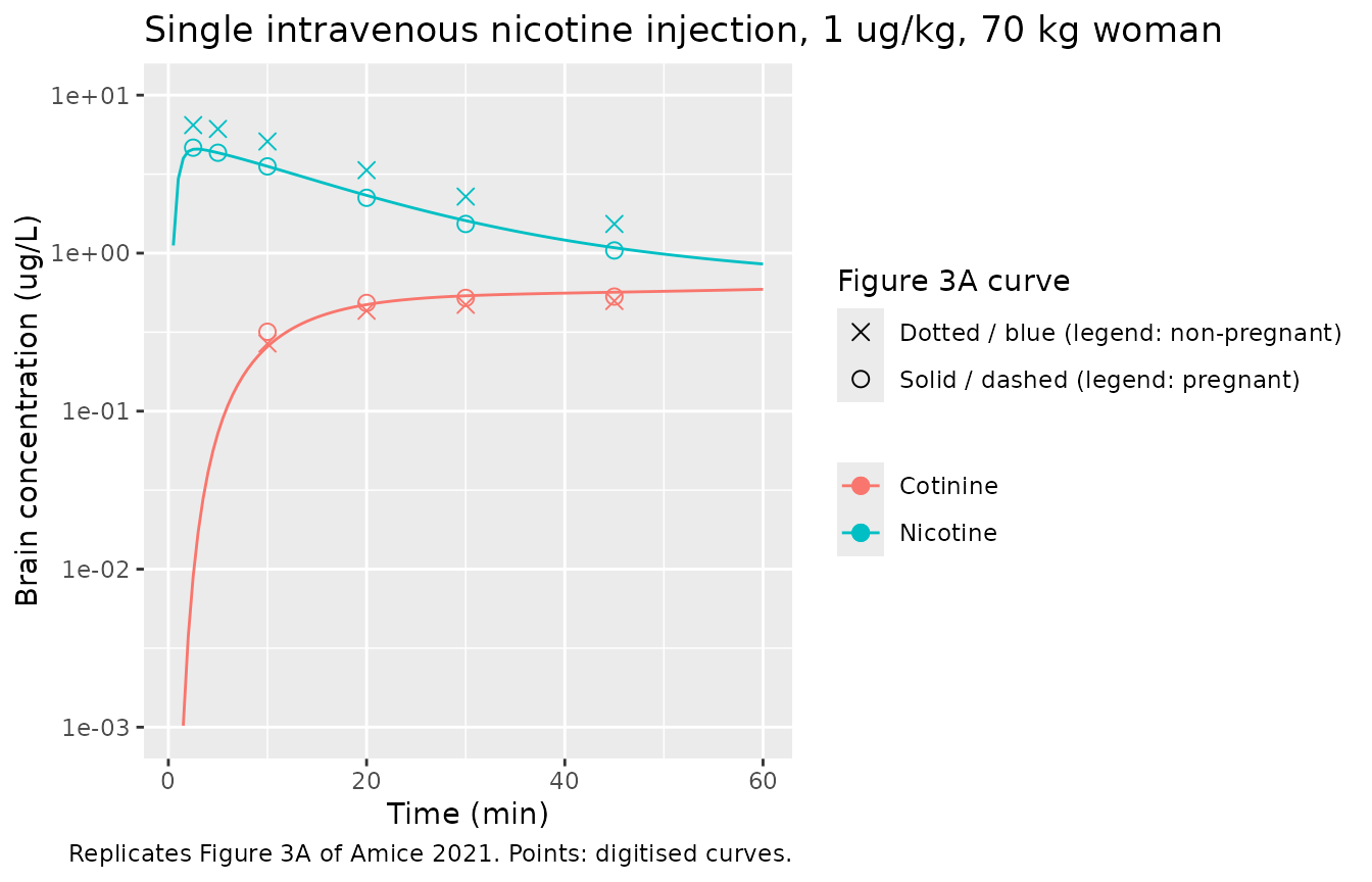
fig3a_cmp |>
  dplyr::mutate(
    model = signif(model, 3),
    dplyr::across(dplyr::starts_with("pct_"), \(x) round(x, 1))
  ) |>
  dplyr::rename(
    "Time (min)" = time_min, "Analyte" = analyte,
    "Solid / dashed (ug/L)" = solid_or_dashed, "Dotted / blue (ug/L)" = dotted_or_blue,
    "Model (ug/L)" = model,
    "Model vs solid / dashed (%)" = pct_vs_solid_or_dashed,
    "Model vs dotted / blue (%)" = pct_vs_dotted_or_blue
  ) |>
  knitr::kable(caption = "Model brain concentrations against the digitised Figure 3A curves.")

Model brain concentrations against the digitised Figure 3A curves.

Time (min)	Analyte	Solid / dashed (ug/L)	Dotted / blue (ug/L)	Model (ug/L)	Model vs solid / dashed (%)	Model vs dotted / blue (%)
2.5	Nicotine	4.650	6.460	4.540	-2.4	-29.7
5.0	Nicotine	4.320	6.110	4.320	-0.1	-29.3
10.0	Nicotine	3.540	5.090	3.540	0.1	-30.4
20.0	Nicotine	2.240	3.350	2.320	3.6	-30.7
30.0	Nicotine	1.530	2.280	1.610	5.0	-29.6
45.0	Nicotine	1.040	1.530	1.080	4.1	-29.3
10.0	Cotinine	0.318	0.268	0.256	-19.4	-4.3
20.0	Cotinine	0.484	0.432	0.472	-2.4	9.3
30.0	Cotinine	0.521	0.471	0.537	3.1	14.0
45.0	Cotinine	0.531	0.498	0.566	6.6	13.6

tmax_brain_min <- 60 * sim_bolus$time[which.max(sim_bolus$Cbrain)]
c(peak_brain_nicotine = max(sim_bolus$Cbrain), tmax_min = tmax_brain_min)
#> peak_brain_nicotine            tmax_min 
#>            4.555099            3.000000

# Model brain nicotine reproduces the SOLID curve at every digitised point
# (observed -2.4% to +5.0%); see the deviations for why the legend calls it
# the pregnant curve. The digitised peak of both curves is at 2.5-3 min; the
# text says 'within 2 min'.
nic3a <- dplyr::filter(fig3a_cmp, analyte == "Nicotine")
stopifnot(
  max(abs(nic3a$pct_vs_solid_or_dashed)) < 10,
  tmax_brain_min <= 3
)

PKNCA validation

The paper reports a nicotine peak at about 1 h, a nicotine half-life of about 3 h and a cotinine half-life of about 16 h (Results, “Baseline PBPK Model”). The nicotine values come from the 5-h window of Figure 2A; the cotinine half-life is taken from the 24-h cotinine infusion of Figure 2B.

nca_input <- dplyr::bind_rows(
  sim_nic |>
    dplyr::filter(time <= 5) |>
    dplyr::transmute(id = 1L, time, Cc, treatment = "Nicotine, nicotine infusion"),
  sim_cot |>
    dplyr::transmute(id = 2L, time, Cc = Cc_cot, treatment = "Cotinine, cotinine infusion")
) |>
  dplyr::filter(!is.na(Cc))

conc_obj <- PKNCA::PKNCAconc(nca_input, Cc ~ time | treatment + id)
dose_df <- tibble::tibble(
  id = c(1L, 2L), time = 0, amt = c(600, 20100),
  treatment = c("Nicotine, nicotine infusion", "Cotinine, cotinine infusion")
)
dose_obj <- PKNCA::PKNCAdose(dose_df, amt ~ time | treatment + id)

intervals <- data.frame(start = 0, end = Inf, cmax = TRUE, tmax = TRUE, half.life = TRUE)
nca_res <- PKNCA::pk.nca(PKNCA::PKNCAdata(conc_obj, dose_obj, intervals = intervals))

Comparison against the published values

published <- tibble::tribble(
  ~treatment,                     ~tmax, ~half.life,
  "Nicotine, nicotine infusion",  1,     3,
  "Cotinine, cotinine infusion",  NA,    16
)

cmp <- nlmixr2lib::ncaComparisonTable(
  simulated = nca_res,
  reference = published,
  by = "treatment",
  params = c("tmax", "half.life"),
  units = c(tmax = "h", half.life = "h"),
  tolerance_pct = 20
)
knitr::kable(cmp, caption = "Simulated against published values. * differs from reference by >20%.")

Simulated against published values. * differs from reference by >20%.

NCA parameter	treatment	Reference	Simulated	% diff
Tmax (h)	Nicotine, nicotine infusion	1	1	+0.0%
Tmax (h)	Cotinine, cotinine infusion	—	0.5	—
t½ (h)	Nicotine, nicotine infusion	3	2.97	-0.9%
t½ (h)	Cotinine, cotinine infusion	16	13.5	-15.4%

res <- as.data.frame(nca_res$result)
get_par <- function(trt, par) res$PPORRES[res$treatment == trt & res$PPTESTCD == par]
stopifnot(
  abs(get_par("Nicotine, nicotine infusion", "tmax") - 1) < 0.1,
  abs(get_par("Nicotine, nicotine infusion", "half.life") / 3 - 1) < 0.2,
  abs(get_par("Cotinine, cotinine infusion", "half.life") / 16 - 1) < 0.2
)

The nicotine peak time and half-life agree with the paper. The cotinine half-life is shorter than the rounded “~16 h” of the text but matches the terminal slope of the authors’ own Figure 2B curve (previous section), which is about 13-14 h.

Assumptions and deviations

• Only the non-pregnant baseline model is packaged. The pregnancy model could not be reproduced from the published material, for five reasons:
  1. The main text and Table S.2 describe placental transfer as an influx-efflux model with four transfer constants Kt1-Kt4 (1500, 1000, 880 and 1000 L/h), but none of Kt1-Kt4 appears in the 32 printed equations. The placental and fetal-blood equations (DS1 Eqs 23, 24, 28 and 32) instead use a Michaelis-Menten exchange term scaled by a coefficient PAF.
  2. PAF, the placental partition coefficients and the fetal cardiac output (printed as “FQblood-fetus = L/h/kg”, with no number) are not given anywhere. The fetal blood fraction is 0.0085 on the equations page and 0.085 in Table S.2.
  3. The printed equations have defects: Eq 24 (placental cotinine) uses the arterial nicotine concentration, the venous equations have no placental return, and the “fetal clearance 20% of maternal” assumption of the Results has no term in fetal Eqs 25-32.
  4. The “muscle clearance” update mentioned in the Methods has no value.
  5. Swapping in only the pregnant clearances of Table 1 (column 3) at 73 kg lowers plasma nicotine and cotinine at 150 min by about 22% and 1%. The paper reports about 70% and 30%, so a mother-only pregnant variant would not reproduce the paper and is not offered. The pregnancy model will be added if the authors’ MATLAB code becomes available.
• Mammary and uterus compartments are omitted. They appear in DS1 Eqs 6-7 and 17-18 but are pregnancy compartments (Table S.2); the adult Table S.1 lists no volume or flow for them, and the adult flow fractions already sum to 1.
• The infusion compartment Vit is not implemented. Table S.1 lists a Vit volume (0.0214 of body weight) and Table S.3 a transfer rate Kvit of 4.1 /min, but no equation uses them: Eq 11 doses the venous blood directly. The model follows the equations.
• Plasma versus blood. The equations track blood. Cc and Cc_cot are blood divided by the Table S.3 blood:plasma ratios (0.8 and 0.88), the reading that matches the post-infusion curves of Figure 2A. Whole-blood outputs Cblood and Cblood_cot are also returned.
• Nicotine during the infusion. Up to the end of the nicotine infusion, the authors’ Figure 2A curve rises more slowly than this model: about 2.1 vs 4.3 ug/L at 15 min, and a peak of about 5.5 vs 7.5 ug/L at 60 min. From 100 min on the two agree within digitisation error, and the paper’s printed urinary recoveries are reproduced. The published equations do not explain the early difference. Reading Kvit as 4.1 /h instead of 4.1 /min reproduces the first 15 min but overshoots every later point, so the maintainers did not adopt it.
• Cotinine level after the cotinine infusion. The authors’ Figure 2B model curve is about 20% below this model’s whole-blood cotinine and about 30% below its plasma cotinine at every time after 1 h, with the same terminal slope. This model’s whole-blood cotinine lies close to De Schepper’s observed data. The published material does not explain the offset. The figure title gives the infusion rate as 0.65 mg/min and the text as 0.67 mg/min; the text value is used, and the 3% difference does not account for the offset.
• Figure 3A brain nicotine. This non-pregnant model reproduces the solid nicotine curve of Figure 3A within about 5% at every digitised point. The figure legend assigns that curve to the pregnant woman and the dotted curve, about 1.4 times higher, to the non-pregnant woman. The maintainers could not determine whether the line styles in the legend are swapped. The two curves also differ much less than the pregnant and non-pregnant plasma curves of Figure 2A (about 0.7 vs 0.3 at comparable times), so Figure 3A cannot settle the question. The model brain cotinine lies within about 20% of both cotinine curves.
• Clearance units and the “men” column. The clearances are the women’s values of Table 1 (mL/min/kg), multiplied by body weight. The “men” column (Curvall 1990 / Robinson 1992) is printed in mL/h/kg in Table 1 but in kg^0.25/h and L/h/kg^0.75 in Table S.1. It is not used, because the paper’s baseline is a woman. The Figure 2A caption says “adult men”, but its title says “adult female plasma”, and the women’s clearances reproduce the paper’s urinary recoveries.
• Cotinine formation on a mass basis. Eq 20 forms cotinine at 0.8 times the hepatic nicotine elimination rate in mass units, with no correction for the molecular weights (162.2 and 176.2 g/mol). The model follows the equation.
• No variability. The paper reports no between-subject variability and no residual error, so none is declared.
• Digitised values. The Figure 2A, 2B and 3A values above were digitised by the maintainers from the published figures. They carry a reading uncertainty of a few percent.
• No correction notice for the article was found on the journal page or in PubMed as of 2026-10-16.