Rifampicin (Marsot 2017)
Source:vignettes/articles/Marsot_2017_rifampicin.Rmd
Marsot_2017_rifampicin.RmdModel and source
- Citation: Marsot A, Menard A, Dupouey J, Muziotti C, Guilhaumou R, Blin O. Population pharmacokinetics of rifampicin in adult patients with osteoarticular infections: interaction with fusidic acid. Br J Clin Pharmacol. 2017 May;83(5):1039-1047. doi:10.1111/bcp.13178.
- Description: One-compartment population pharmacokinetic model for oral rifampicin in adult patients with staphylococcal osteoarticular infections (Marsot 2017; 62 patients, 103 steady-state plasma concentrations from routine therapeutic drug monitoring at 300 mg three times daily). Absorption uses a single-transit compartment chain (depot -> transit1 -> central) with a fixed first-order absorption rate constant ka = 1.15 1/h; first-order elimination from the central compartment. Coadministration of oral fusidic acid (500 mg three times daily in 16 % of the cohort) was retained as the sole significant covariate and reduces both apparent oral clearance and apparent central volume of distribution: typical CL/F is 5.1 L/h (with fusidic acid) vs 13.7 L/h (without) and typical V/F is 23.8 L (with) vs 61.1 L (without), an interaction attributed to CYP3A4 inhibition and altered plasma protein binding by fusidic acid. Inter-individual variability is reported on CL/F (72.9 % CV) and V/F (59.1 % CV); residual variability is additive with standard deviation 2.256 mg/L.
- Article: Br J Clin Pharmacol 2017;83(5):1039-1047
Population
Marsot 2017 fitted the model to routine therapeutic-drug-monitoring (TDM) samples from 62 adult outpatients with staphylococcal osteoarticular infections at Conception Hospital in Marseille, France (mean age 57.4 years, range 20-89; mean weight 72.3 kg, range 46-119; 25.8 % female; Table 1). All patients received oral rifampicin 300 mg three times daily for 3 months (soft-tissue infections) or 6 months (infections associated with prosthetic materials). 75.8 % of the cohort had a prosthesis or osteosynthesis in place. Concomitant antibiotics included ofloxacin (51.6 %), fusidic acid (16.1 %), clindamycin (9.7 %), teicoplanin (9.7 %), and several others; of these, only oral fusidic acid (500 mg three times daily) was retained as a significant covariate in the final model. Only steady-state samples (drawn less than 4 weeks after treatment start) were included, yielding 103 plasma rifampicin observations quantified by HPLC-UV (LLOQ 0.5 mg/L).
The same information is available programmatically via
readModelDb("Marsot_2017_rifampicin")()$population.
Source trace
Every ODE, algebraic assignment, and ini() parameter has
an in-file source-trace comment in
inst/modeldb/specificDrugs/Marsot_2017_rifampicin.R. The
table below collects them in one place.
| Equation / parameter | Value | Source location |
|---|---|---|
| Structural model (1-cpt + single transit + first-order elim) | n/a | Results paragraph 2 and Figure 1 caption (“Representation of the final model”) |
lcl (CL/F without fusidic acid, L/h) |
log(13.7) | Table 2 row “CL/F (l h^-1) Without fusidic acid” = 13.7 (RSE 26.3 %) |
lvc (V/F without fusidic acid, L) |
log(61.1) | Table 2 row “V/F (l) Without fusidic acid” = 61.1 (RSE 56.5 %) |
lka (ka, 1/h; fixed) |
fixed(log(1.15)) | Results paragraph 2 and Discussion paragraph 4: “the absorption rate constant was fixed at 1.15 h^-1 to improve the fit” |
lfdepot (F, fixed anchor) |
fixed(log(1)) | Standard oral-only apparent parameterisation; no F estimated |
e_conmed_fusidic_cl |
log(5.1 / 13.7) = -0.988 | Table 2 row “CL/F With / Without” = 5.1 / 13.7 |
e_conmed_fusidic_vc |
log(23.8 / 61.1) = -0.943 | Table 2 row “V/F With / Without” = 23.8 / 61.1 |
IIV etalcl (variance on log scale) |
0.531 | Table 2 row “omega CL/F” = 0.531 (RSE 38.3 %); consistent with abstract 72.9 % CV |
IIV etalvc (variance on log scale) |
0.349 | Table 2 row “omega V/F” = 0.349 (RSE 238.1 %); consistent with abstract 59.1 % CV |
addSd (additive residual SD, mg/L) |
2.256 | Table 2 row “sigma_add (mg l^-1)” = 2.256 (RSE 12.4 %); abstract “2.3 mg l^-1” |
ODE: d/dt(depot) <- -ka * depot
|
n/a | Methods paragraph “Absorption … was modelled using transit compartments” |
ODE: d/dt(transit1) <- ka * (depot - transit1)
|
n/a | Methods paragraph and Discussion paragraph 4 (single-transit chain, N = 1) |
ODE:
d/dt(central) <- ka * transit1 - kel * central
|
n/a | Methods paragraph “Elimination was assumed to take place from the central plasma compartment” |
Cc <- central / vc |
n/a | Standard apparent-volume normalisation of central amount to plasma concentration |
Residual Cc ~ add(addSd)
|
n/a | Methods paragraph “an additive error model … C_ij = CP_ij + epsilon_ij” |
Virtual cohort
Original observed rifampicin concentrations are not publicly available. The figures below simulate a virtual cohort whose covariate structure approximates Marsot 2017 Table 1: two strata of 100 subjects each, CONMED_FUSIDIC = 0 (rifampicin monotherapy) and CONMED_FUSIDIC = 1 (rifampicin + fusidic acid coadministration). The stratum split matches the paper’s contrast rather than the cohort proportions (16.1 % on fusidic acid), so that both strata are precision-simulated.
set.seed(20250701)

n_per_arm <- 100L

# Steady-state dosing window: 300 mg TID (q8h), sample over one dose
# interval (0-8 h post-dose) at steady state, plus a short extension
# to 12 h so both the peak and the terminal-phase decline can be
# inspected. Steady state is achieved via ss = 1 on the first dose,
# using rxode2's built-in extravascular steady-state prime.
sample_times <- seq(0, 12, by = 0.25)

make_cohort <- function(n, fusidic, id_offset) {
  subj <- tibble(id = id_offset + seq_len(n), CONMED_FUSIDIC = fusidic)
  dose <- subj |> mutate(time = 0, amt = 300, evid = 1, cmt = "depot",
                         ii = 8, ss = 1L)
  obs  <- subj |> tidyr::crossing(time = sample_times) |>
    mutate(amt = NA_real_, evid = 0L, cmt = "central", ii = 0, ss = 0L)
  bind_rows(dose, obs) |>
    mutate(treatment = if (fusidic == 1L) "Rifampicin + fusidic acid"
                       else                "Rifampicin alone") |>
    arrange(id, time, desc(evid))
}

events <- bind_rows(
  make_cohort(n_per_arm, fusidic = 0L, id_offset =   0L),
  make_cohort(n_per_arm, fusidic = 1L, id_offset = n_per_arm)
)

stopifnot(!anyDuplicated(unique(events[, c("id", "time", "evid")])))
Simulation
mod <- readModelDb("Marsot_2017_rifampicin")

sim <- rxode2::rxSolve(
  mod, events = events,
  keep = c("treatment", "CONMED_FUSIDIC"),
  # steady-state searches for long-half-life subjects exceed the default step budget
  maxsteps = 1e6
) |> as.data.frame()
For deterministic typical-value replication of the two strata, zero out the IIV:
mod_typical <- mod |> rxode2::zeroRe()

sim_typical <- rxode2::rxSolve(
  mod_typical,
  events = events |> dplyr::filter(id %in% c(1L, n_per_arm + 1L)),
  keep   = c("treatment", "CONMED_FUSIDIC"),
  # steady-state searches for long-half-life subjects exceed the default step budget
  maxsteps = 1e6
) |> as.data.frame()
#> ℹ omega/sigma items treated as zero: 'etalcl', 'etalvc'
#> Warning: multi-subject simulation without without 'omega'
Replicate published figures
Marsot 2017 Figure 4 is a prediction-corrected VPC of rifampicin plasma concentration vs. time after dose stratified by fusidic acid coadministration. The panel below reproduces that stratification as a VPC-style ribbon on the simulated cohort.
sim |>
  dplyr::group_by(treatment, time) |>
  dplyr::summarise(
    Q05 = quantile(Cc, 0.05, na.rm = TRUE),
    Q50 = quantile(Cc, 0.50, na.rm = TRUE),
    Q95 = quantile(Cc, 0.95, na.rm = TRUE),
    .groups = "drop"
  ) |>
  ggplot(aes(time, Q50)) +
  geom_ribbon(aes(ymin = Q05, ymax = Q95), alpha = 0.25) +
  geom_line() +
  facet_wrap(~ treatment) +
  labs(x = "Time after dose (h)",
       y = "Rifampicin plasma concentration (mg/L)",
       title = "Simulated VPC at steady state (300 mg q8h)",
       caption = "Replicates the stratification in Figure 4 of Marsot 2017 (fusidic acid: 0 vs 1).")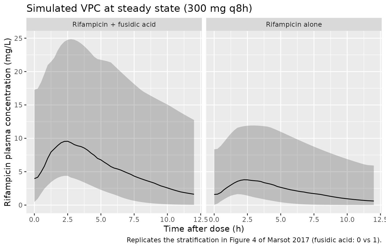
Marsot 2017 Figure 5 presents box plots of the individual (empirical Bayes) CL/F and V/F stratified by fusidic acid coadministration. The plots below replicate that contrast at the individual-parameter level, using the model’s per-subject CL/F and V/F draws from the virtual cohort.
subj_params <- sim |>
  dplyr::distinct(id, treatment, cl, vc)

bind_rows(
  subj_params |> dplyr::mutate(parameter = "CL/F (L/h)", value = cl),
  subj_params |> dplyr::mutate(parameter = "V/F  (L)",   value = vc)
) |>
  ggplot(aes(treatment, value, fill = treatment)) +
  geom_boxplot(alpha = 0.6, outlier.size = 0.5) +
  facet_wrap(~ parameter, scales = "free_y") +
  scale_y_log10() +
  labs(x = NULL, y = NULL,
       title = "Individual PK parameters by fusidic acid coadministration",
       caption = "Replicates the stratification in Figure 5 of Marsot 2017.") +
  theme(legend.position = "none")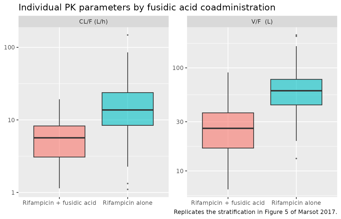
PKNCA validation
Marsot 2017 does not tabulate NCA parameters. Two independent validation checks are performed instead:
- The steady-state analytical relationships (Css,avg = Dose / (CL * tau)) for each stratum, using the paper’s Table 2 typical values.
- PKNCA-derived Cmax, Tmax, AUC, and half-life on the simulated typical-value profiles, compared against the analytical predictions so that any discrepancy points to an implementation error in the model file rather than to a paper-vs-simulation mismatch.
# Use the typical-value simulation for a paper-vs-model NCA comparison.
sim_nca <- sim_typical |>
  dplyr::filter(!is.na(Cc)) |>
  dplyr::select(id, time, Cc, treatment)

# Guarantee a time-zero row per (id, treatment) so PKNCA can anchor
# AUC0-* for the steady-state (0 to 8 h) window.
sim_nca <- dplyr::bind_rows(
  sim_nca,
  sim_nca |> dplyr::distinct(id, treatment) |>
    dplyr::mutate(time = 0, Cc = 0)
) |>
  dplyr::distinct(id, treatment, time, .keep_all = TRUE) |>
  dplyr::arrange(id, treatment, time)

conc_obj <- PKNCA::PKNCAconc(sim_nca, Cc ~ time | treatment + id)

dose_df <- events |>
  dplyr::filter(evid == 1L, id %in% c(1L, n_per_arm + 1L)) |>
  dplyr::select(id, time, amt, treatment)

dose_obj <- PKNCA::PKNCAdose(dose_df, amt ~ time | treatment + id)

intervals <- data.frame(
  start     = 0,
  end       = 8,
  cmax      = TRUE,
  tmax      = TRUE,
  auclast   = TRUE,
  half.life = TRUE
)

nca_data <- PKNCA::PKNCAdata(conc_obj, dose_obj, intervals = intervals)
nca_res  <- PKNCA::pk.nca(nca_data)
Comparison against analytical steady-state predictions
At steady state, the average concentration over one dose interval is Css,avg = F * Dose / (CL/F * tau). With the Marsot 2017 typical values and tau = 8 h:
- No fusidic acid: Css,avg = 300 / (13.7 * 8) = 2.74 mg/L
- With fusidic acid: Css,avg = 300 / (5.1 * 8) = 7.35 mg/L
auclast / 8 should reproduce these numbers within a few
percent (agreement gets tighter as the sampling grid is refined).
nca_summary <- as.data.frame(nca_res$result) |>
  dplyr::select(treatment, PPTESTCD, PPORRES) |>
  tidyr::pivot_wider(names_from = PPTESTCD, values_from = PPORRES) |>
  dplyr::mutate(Css_avg = auclast / 8)

published <- tibble::tribble(
  ~treatment,                   ~cl_lhr, ~vc_l, ~Css_avg_analytical,
  "Rifampicin alone",           13.7,    61.1,  300 / (13.7 * 8),
  "Rifampicin + fusidic acid",   5.1,    23.8,  300 /  (5.1 * 8)
)

comparison <- nca_summary |>
  dplyr::left_join(published, by = "treatment") |>
  dplyr::select(treatment, cmax, tmax, auclast, half.life, Css_avg, Css_avg_analytical) |>
  dplyr::mutate(
    dplyr::across(where(is.numeric), ~ round(.x, 3))
  )

comparison |>
  dplyr::rename(
    "Stratum"                            = treatment,
    "Cmax (mg/L)"                        = cmax,
    "Tmax (h)"                           = tmax,
    "AUC0-8 (mg*h/L)"                    = auclast,
    "t1/2 (h)"                           = half.life,
    "Css,avg PKNCA (mg/L)"               = Css_avg,
    "Css,avg analytical (mg/L)"          = Css_avg_analytical
  ) |>
  knitr::kable(
    caption = "Steady-state NCA on the typical-value simulation vs the analytical Css,avg from Marsot 2017 Table 2 (300 mg q8h). PKNCA and analytical Css,avg should agree within a few percent."
)| Stratum | Cmax (mg/L) | Tmax (h) | AUC0-8 (mg*h/L) | t1/2 (h) | Css,avg PKNCA (mg/L) | Css,avg analytical (mg/L) |
|---|---|---|---|---|---|---|
| Rifampicin + fusidic acid | 10.002 | 2.5 | 58.818 | 3.357 | 7.352 | 7.353 |
| Rifampicin alone | 3.771 | 2.5 | 21.896 | 3.211 | 2.737 | 2.737 |
Assumptions and deviations
-
Residual-error interpretation. Marsot 2017
Materials and method writes the residual model as
C_ij = CP_ij + epsilon_ij(additive in linear space), while Results paragraph 2 describes it as “an additive model on natural log-transformed data” (which usually maps to proportional / exponential residual in linear space). Table 2 reportssigma_add = 2.256 mg/L(with mg/L units) and the abstract summarises “Residual variability was 2.3 mg l^-1 (1.6, 2.6 mg l^-1)”. The linear units in Table 2 and the abstract only make sense if 2.256 is a standard deviation in linear-concentration units, so the model implementsCc ~ add(addSd)withaddSd = 2.256. The “additive on natural log-transformed data” language in Results paragraph 2 is read as a description of the goodness-of-fit diagnostic used to select the residual form rather than a statement about the equation implemented. The Table 2 footnote’s “sigma, variance of epsilon_ij” description is inconsistent with the reported units and with the omega diagonals (whose 0.531 and 0.349 values reproduce the abstract CVs exactly only under a variance interpretation), which supports the reading that Table 2 mixes conventions between omega (variances) and sigma (SD). -
Encoding of the fusidic acid covariate effect.
Marsot 2017 Table 2 reports separate typical CL/F and V/F values for the
two fusidic-acid strata rather than a multiplicative coefficient. This
extraction rewrites the stratification as log-scale offsets
e_conmed_fusidic_cl = log(5.1 / 13.7)ande_conmed_fusidic_vc = log(23.8 / 61.1)applied per-subject viaCONMED_FUSIDIC, exactly reproducing the paper’s typical values atCONMED_FUSIDIC= 0 and 1. No new information is introduced; the representation is chosen for compatibility with the standard covariate-effect naming in the nlmixr2lib register. -
Transit compartment structure. The paper reports
“one transit compartment” between the depot and the central compartment,
with a “final transit compartment feeding an absorption compartment at
rate ka”. The Savic-style implementation used here places one
intermediate compartment (
transit1) betweendepotandcentral, with the same rate constantka = 1.15 1/happlied todepot -> transit1and totransit1 -> central, matching the two-step first-order chain used elsewhere in nlmixr2lib for a single-transit rifampicin absorption (e.g.Svensson_2016_rifampicin.R). -
Covariates evaluated but not retained. Marsot 2017
evaluated age, weight, height, and sex but did not retain any of them in
the final model (Results paragraph 3: “The other covariables tested on
the model, including gender, age, height and body weight, did not
improve the pharmacokinetic model.”). These are recorded as
covariatesDataExcludedmetadata in the model file so downstream users can see they were screened without introducing convention warnings about declared-but-unused covariates. - Auto-induction and nonlinear elimination. Marsot 2017 explicitly tested and rejected a well-stirred-liver auto-induction model (per Chirehwa 2017) and a Michaelis-Menten elimination model in favour of the linear one-compartment model reported here. Rationale in the paper: only steady-state samples (i.e. after auto-induction has plateaued) were used, and the median dose of 12.4 mg/kg is below the 20 mg/kg threshold at which nonlinear rifampicin PK has been observed. Downstream users who want to simulate a non-steady-state or high-dose scenario should instead reach for a rifampicin model that includes auto-induction (e.g. Smythe 2012 / Svensson 2016).
- Directional interpretation of the fusidic acid effect. The paper’s Conclusion states “This concomitant administration induced a significant increase in rifampicin CL/F and V/F”. This wording is inconsistent with Table 2 (CL/F 5.1 with fusidic acid vs 13.7 without; V/F 23.8 vs 61.1) and with the rest of the paper’s narrative (“Patients cotreated with fusidic acid presented an important decrease in the CL and V/F of rifampicin: 5.1 l h^-1 vs 13.7 l h^-1 and 23.8 l vs 61.1 l, respectively”, Discussion paragraph 3). The model uses the numeric values in Table 2 (fusidic acid decreases both CL/F and V/F, yielding higher steady-state rifampicin exposure), consistent with the paper’s “potentially supratherapeutic rifampicin concentrations” conclusion.