Difloxacin in crucian carp (Ma 2023)
Source:vignettes/articles/Ma_2023_difloxacin_crucianCarp.Rmd
Ma_2023_difloxacin_crucianCarp.RmdModel and source
#> ℹ parameter labels from comments will be replaced by 'label()'- Citation: Ma K-L, Yang F, Zhang M, Chen J-C, Duan M-H, Li Z-E, Dai Y, Liu Y, Jin Y-G, Yang F. (2023). Population Pharmacokinetics of Difloxacin in Crucian Carp (Carassius auratus) after a Single Oral Administration. Veterinary Sciences 10(7):416. doi:10.3390/vetsci10070416.
- Article: https://doi.org/10.3390/vetsci10070416
- Open access full text (PMC): https://www.ncbi.nlm.nih.gov/pmc/articles/PMC10383650/
Veterinary (crucian carp, Carassius auratus). One-compartment population PK model with first-order absorption and no absorption lag for difloxacin after a single 20 mg/kg body-weight oral (gavage) dose in crucian carp held at 21.3 +/- 1.2 degC. Ma 2023 fitted 25 sparsely sampled fish (three plasma samples each, drawn from a 15-point 0.25-120 h grid) in Phoenix NLME 8.1. Doses, clearance and volume are all body-weight normalised in the source (dose in mg/kg, tvV in L/kg, tvCL in L/h/kg), so the model is driven with amt in mg/kg and returns Cc directly in ug/mL. Final (‘covariance’) model, Table 3: tvKa 1.18 1/h, tvV 14.18 L/kg, tvCL 0.20 L/h/kg, with exponential between-fish variability on all three (omega^2 = 0.69, 1.12 and 0.98) and a Phoenix log-additive residual error, stdev0 = 0.16 on the log scale, encoded as lnorm(expSd). Body weight was screened as a covariate on CL/F, V/F and Ka and rejected (delta -2LL = 3.02, below the 6.64 significance threshold), so no covariate enters the model. The authors fitted a FULL variance-covariance omega block over etaKa, etaV and etaCL but published only the three diagonal variances; the off-diagonals are therefore absent here and the etas are independent. See the vignette for the consequences.
Ma 2023 is, in the authors’ words, the first population PK analysis of difloxacin in crucian carp. Difloxacin is a third-generation fluoroquinolone used extra-label in Chinese aquaculture; no fish-specific dosing guidance exists, so mammalian regimens are extrapolated. The paper’s practical conclusion is that the 20 mg/kg oral dose in current use does not reach a free AUC/MIC of 125 against Aeromonas hydrophila.
Population
Thirty healthy crucian carp (Carassius auratus) were split into six equal groups of five; one group was an undosed control supplying blank plasma, leaving 25 dosed fish (Section 2.2). Mean body weight was 0.298 kg (range 0.21 to 0.40 kg; per-fish weights are listed in Table 1). Fish were held at 21.3 +/- 1.2 degC after at least 10 days of acclimation, in water at pH ~7.4 with dissolved oxygen above 7.5 mg/L.
Each fish received a single 20 mg/kg body-weight oral gavage dose of difloxacin hydrochloride (10 mg/mL in 0.9% saline) and was sampled sparsely, three times only, from the tail vein. Table 1 shows five repeating three-point schedules cycling across the 25 fish, between them covering all 15 nominal sampling times from 0.25 to 120 h. Plasma difloxacin was measured by HPLC-UV at 276 nm (calibration 0.1 to 5 ug/mL, LOQ 0.1 ug/mL).
The same information is available programmatically via the model’s
population metadata:
str(ui$population)
#> List of 14
#>  $ species          : chr "crucian carp (Carassius auratus)"
#>  $ n_subjects       : int 25
#>  $ n_studies        : int 1
#>  $ weight_range     : chr "0.21-0.40 kg"
#>  $ weight_mean      : chr "0.298 kg"
#>  $ dose_range       : chr "single 20 mg/kg body weight oral gavage (10 mg/mL difloxacin hydrochloride in 0.9% saline)"
#>  $ disease_state    : chr "healthy"
#>  $ regions          : chr "China (Henan University of Science and Technology, Luoyang)"
#>  $ water_temperature: chr "21.3 +/- 1.2 degC"
#>  $ water_quality    : chr "pH ~7.4; total ammonia nitrogen <= 0.7 mg/L; nitrite nitrogen < 0.07 mg/L; dissolved oxygen > 7.5 mg/L"
#>  $ design           : chr "30 fish in 6 equal groups of 5; one group served as an undosed control supplying blank plasma, leaving 25 dosed"| __truncated__
#>  $ sampling         : chr "Sparse: each dosed fish sampled 3 times from the tail vein. Table 1 shows five repeating schedules of three tim"| __truncated__
#>  $ bioanalysis      : chr "HPLC-UV at 276 nm; calibration 0.1-5 ug/mL, LOQ 0.1 ug/mL, mean recovery 81.46%, intra-day CV 0.74-7.72%, inter"| __truncated__
#>  $ notes            : chr "Baseline weights are listed per fish in Table 1; the group description is in Section 2.2. Only one water temper"| __truncated__
Study design (Ma 2023 Table 1)
The sparse-sampling design is reproduced below exactly as printed, and is used later to evaluate the model on the paper’s own measurement grid rather than on a finer grid of our choosing.
# Ma 2023 Table 1: per-fish body weight and the three sampling times.
# The five schedules cycle in order across fish 1..25.
schedules <- list(
  A = c(0.25, 6, 36),
  B = c(0.5, 8, 48),
  C = c(1, 12, 72),
  D = c(2, 16, 96),
  E = c(4, 24, 120)
)
table1 <- tibble::tibble(
  id = 1:25,
  # Ma 2023 Table 1, BW (kg) column, in printed ID order
  WT = c(0.21, 0.33, 0.37, 0.35, 0.31, 0.26, 0.28, 0.26, 0.27, 0.27,
         0.30, 0.27, 0.34, 0.23, 0.40, 0.25, 0.28, 0.27, 0.29, 0.36,
         0.33, 0.29, 0.29, 0.34, 0.31),
  schedule = rep(names(schedules), times = 5)
)

# The 15 nominal times of Section 2.3, each covered by exactly 5 fish.
nominal_times <- c(0.25, 0.5, 1, 2, 4, 6, 8, 12, 16, 24, 36, 48, 72, 96, 120)
covered <- sort(unlist(schedules, use.names = FALSE))
stopifnot(
  nrow(table1) == 25L,
  # Section 2.2: 30 fish in 6 groups of 5, one group is the undosed control.
  nrow(table1) == 30L - 5L,
  # Section 2.3: "Each fish was sparsely sampled three times".
  all(lengths(schedules) == 3L),
  setequal(covered, nominal_times),
  # Weight range and mean quoted in Section 2.2.
  min(table1$WT) == 0.21, max(table1$WT) == 0.40,
  abs(mean(table1$WT) - 0.298) < 0.005
)
c(n_fish = nrow(table1), n_samples = nrow(table1) * 3L,
  mean_WT = round(mean(table1$WT), 3))
#>    n_fish n_samples   mean_WT
#>    25.000    75.000     0.298
The printed Table 1 carries 74 asterisks rather than 75: fish 1 shows marks only at 6 and 36 h. Section 2.3 states unambiguously that each fish was sampled three times, and every other fish following schedule A carries the 0.25 h mark, so the missing mark is read here as a typesetting omission.
Source trace
Every value below also carries an in-file comment next to its
ini() entry in
inst/modeldb/specificDrugs/Ma_2023_difloxacin_crucianCarp.R.
| Equation / parameter | Value | Source location |
|---|---|---|
lka (tvKa) |
1.18 1/h | Table 3, Final model (Covariance model) row; RSE 12.55%, CI 0.88 to 1.47 |
lvc (tvV, V/F) |
14.18 L/kg | Table 3, Final model row; RSE 18.88%, CI 8.83 to 19.53 |
lcl (tvCL, CL/F) |
0.20 L/h/kg | Table 3, Final model row; RSE 17.96%, CI 0.13 to 0.27 |
etalka variance |
0.69 | Table 3, “Inter-Individual Variation omega^2 (RSE%)” column, Final model; RSE 35.14% |
etalvc variance |
1.12 | Table 3, same column, Final model; RSE 28.54% |
etalcl variance |
0.98 | Table 3, same column, Final model; RSE 27.08% |
expSd (stdev0) |
0.16 | Table 3, Final model; RSE 11.06%, CI 0.12 to 0.19. Log-additive error model per Section 2.5 |
| One compartment, first-order oral absorption, no lag | n/a | Section 2.5 (Ka / V / CL parameterisation, Phoenix NLME 8.1); Equations 1 to 3 |
| Body weight excluded as a covariate | n/a | Section 2.5 and Section 3.3: delta -2LL = 3.02 < 6.64 |
| Dose 20 mg/kg BW, single oral gavage | n/a | Section 2.3 |
Values in the packaged model come from the final (covariance) model, not the basic model. For reference the basic model gave tvKa 1.16, tvV 14.34, tvCL 0.18, stdev0 0.19.
The residual error model
Section 2.5 states that “the log-additive error model was used”.
Phoenix NLME’s log-additive model is CObs = C * exp(eps)
with eps ~ N(0, stdev0^2), i.e. an additive residual on the
natural-log concentration. That is exactly nlmixr2’s
~ lnorm(expSd), so expSd = 0.16 is a
dimensionless log-scale SD. Table 3 prints “ug/mL” in
the Units column for stdev0; that column also mis-assigns
units across the merged parameter rows, and a log-additive SD cannot
carry concentration units, so the printed unit is treated as a reporting
artefact.
Reproducing the paper’s secondary parameters (Table 4)
Section 2.5 defines the secondary parameters by three closed forms:
- Equation 1:
K10 = tvCL / tvV - Equation 2:
T1/2 = ln(2) * tvV / tvCL - Equation 3:
AUC0-inf = Dose / tvCL
Table 4 reports K10 = 0.01 1/h, T1/2 = 50.14 h and AUC0-inf = 102.05 h*ug/mL. Solving the packaged ODE model at its typical values and running PKNCA on the result is a genuine end-to-end check: it exercises the ODE structure, the dosing route, the body-weight-normalised units and the transcribed parameter values against three published numbers.
mod <- readModelDb("Ma_2023_difloxacin_crucianCarp")
mod_typical <- rxode2::zeroRe(mod)
#> ℹ parameter labels from comments will be replaced by 'label()'

# Fine early grid to resolve Tmax (a coarse grid understates AUC),
# then out to 480 h -- nearly 10 elimination half-lives -- so the aucinf
# extrapolation is a small correction rather than the bulk of the estimate.
grid_typical <- sort(unique(c(seq(0, 24, by = 0.05), seq(24, 480, by = 1))))
ev_typical <- rxode2::et(amt = 20, cmt = "depot") |>
  rxode2::et(grid_typical)

sim_typical <-
  rxode2::rxSolve(mod_typical, ev_typical, returnType = "data.frame") |>
  mutate(id = 1L, treatment = "20 mg/kg")
#> ℹ omega/sigma items treated as zero: 'etalka', 'etalvc', 'etalcl'

# Concentrations must stay non-negative or PKNCA's lambda.z log() misbehaves.
stopifnot(all(sim_typical$Cc >= 0))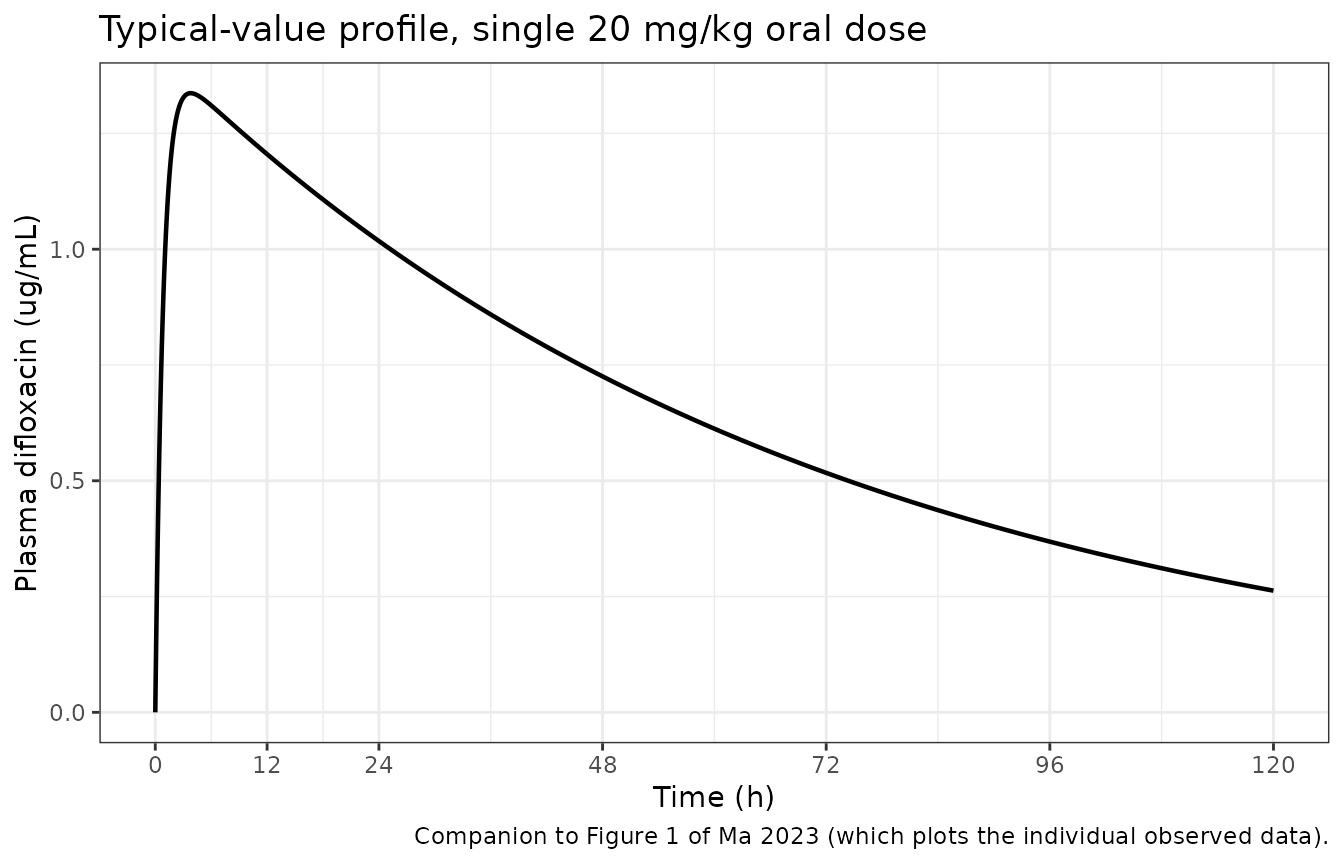
PKNCA validation
nca_conc <- sim_typical |>
  dplyr::filter(!is.na(Cc)) |>
  dplyr::select(id, time, Cc, treatment)

# Guarantee a time = 0 record (extravascular pre-dose Cc = 0).
nca_conc <- dplyr::bind_rows(
  nca_conc,
  nca_conc |> dplyr::distinct(id, treatment) |>
    dplyr::mutate(time = 0, Cc = 0)
) |>
  dplyr::distinct(id, treatment, time, .keep_all = TRUE) |>
  dplyr::arrange(id, treatment, time)

conc_obj <- PKNCA::PKNCAconc(nca_conc, Cc ~ time | treatment + id)

dose_df <- data.frame(id = 1L, time = 0, amt = 20, treatment = "20 mg/kg")
dose_obj <- PKNCA::PKNCAdose(dose_df, amt ~ time | treatment + id)

intervals <- data.frame(
  start = 0, end = Inf,
  cmax = TRUE, tmax = TRUE, auclast = TRUE,
  aucinf.obs = TRUE, half.life = TRUE, lambda.z = TRUE
)

nca_res <- PKNCA::pk.nca(
  PKNCA::PKNCAdata(conc_obj, dose_obj, intervals = intervals)
)

nca_wide <- as.data.frame(nca_res) |>
  dplyr::select(PPTESTCD, PPORRES) |>
  tidyr::pivot_wider(names_from = PPTESTCD, values_from = PPORRES)
nca_wide[, c("cmax", "tmax", "auclast", "aucinf.obs", "half.life", "lambda.z")]
#> # A tibble: 1 × 6
#>    cmax  tmax auclast aucinf.obs half.life lambda.z
#>   <dbl> <dbl>   <dbl>      <dbl>     <dbl>    <dbl>
#> 1  1.34   3.8    99.9      100.0      49.1   0.0141
Gate 1 – Table 4 secondary parameters
auc_sim   <- nca_wide$aucinf.obs
thalf_sim <- nca_wide$half.life
k10_sim   <- nca_wide$lambda.z

pct <- function(sim, ref) (sim - ref) / ref * 100

# Both quantities are DETERMINISTIC (zeroRe: no cohort is drawn), so the
# tolerance is a transcription tolerance, not a sampling tolerance.
#
# Realised: -2.01% on AUC and -2.00% on T1/2, both traceable to a single
# cause -- Table 3 prints tvCL rounded to 2 dp as 0.20, while Table 4's
# AUC0-inf = 102.05 was computed from the unrounded 20/102.05 = 0.19598.
# The packaged model uses the printed 0.20 (see "Assumptions and
# deviations"). A 3% band admits that rounding and nothing else: a 10%
# error in a transcribed clearance, volume, dose or unit moves both
# numbers by 10% or more and turns this red.
stopifnot(
  abs(pct(auc_sim, 102.05)) < 3,
  abs(pct(thalf_sim, 50.14)) < 3,
  # Table 4 prints K10 to 2 dp; the model must round to the same value.
  round(k10_sim, 2) == 0.01
)

tibble::tibble(
  Quantity  = c("AUC0-inf (h*ug/mL)", "T1/2 (h)", "K10 (1/h)"),
  `Ma 2023 Table 4` = c(102.05, 50.14, 0.01),
  Simulated = round(c(auc_sim, thalf_sim, k10_sim), c(2, 2, 4)),
  `% diff`  = round(pct(c(auc_sim, thalf_sim, k10_sim), c(102.05, 50.14, 0.01)), 2)
) |>
knitr::kable(caption = "Gate 1: PKNCA on the typical-value solve vs Ma 2023 Table 4.")| Quantity | Ma 2023 Table 4 | Simulated | % diff |
|---|---|---|---|
| AUC0-inf (h*ug/mL) | 102.05 | 100.0000 | -2.01 |
| T1/2 (h) | 50.14 | 49.1500 | -1.98 |
| K10 (1/h) | 0.01 | 0.0141 | 41.03 |
The residual 2% is fully explained by the printed rounding of
tvCL. Solving for the unrounded values that Table 4 implies
confirms both round back to the values Table 3 prints, so the two tables
are internally consistent and no transcription error is hiding in the
gap:
cl_unrounded <- 20 / 102.05                       # Equation 3 inverted
v_unrounded  <- 50.14 * cl_unrounded / log(2)     # Equation 2 inverted
stopifnot(
  round(cl_unrounded, 2) == 0.20,   # Table 3 prints 0.20
  round(v_unrounded, 2) == 14.18    # Table 3 prints 14.18
)
c(tvCL_implied = round(cl_unrounded, 5), tvV_implied = round(v_unrounded, 4))
#> tvCL_implied  tvV_implied
#>      0.19598     14.17670
Gate 2 – Tmax on the paper’s own sampling grid
Table 2 reports Tmax = 4.00 h from the naive-averaged data. That value can only ever be one of the 15 nominal sampling times, so the correct comparison restricts the model to the paper’s measurement grid rather than to the fine grid used above.
on_grid <- sim_typical |> dplyr::filter(time %in% nominal_times)
stopifnot(nrow(on_grid) == length(nominal_times))
tmax_grid <- on_grid$time[which.max(on_grid$Cc)]

# Exact: the model's peak must land on the same nominal time the paper
# reports. The true continuous Tmax is 3.80 h, and 4 h is its nearest
# neighbour on the grid; a mis-transcribed Ka moves the peak to 2 or 6 h.
stopifnot(tmax_grid == 4)
c(tmax_on_paper_grid = tmax_grid, tmax_continuous = round(nca_wide$tmax, 2))
#> tmax_on_paper_grid    tmax_continuous
#>                4.0                3.8
Comparison against the published NCA
# Ma 2023 reports two NCA-style parameter sets. Table 4 holds the secondary
# parameters DERIVED FROM THE FINAL MODEL, which is the like-for-like
# reference for a simulation from that model. Table 2's Cmax and Tmax are
# the only published values for those two parameters and come from a
# naive-averaged-data NCA, which the authors used only to seed initial
# estimates (Discussion, paragraph 1) -- they are shown here for context and
# are expected to differ.
published <- tibble::tribble(
  ~treatment,  ~cmax, ~tmax, ~aucinf.obs, ~half.life,
  "20 mg/kg",  1.13,  4.00,  102.05,      50.14
)

simulated <- nca_wide |>
  dplyr::mutate(treatment = "20 mg/kg") |>
  dplyr::select(treatment, cmax, tmax, aucinf.obs, half.life)

cmp <- nlmixr2lib::ncaComparisonTable(
  simulated     = simulated,
  reference     = published,
  by            = "treatment",
  units         = c(cmax = "ug/mL", tmax = "h",
                    aucinf.obs = "h*ug/mL", half.life = "h"),
  tolerance_pct = 20
)

knitr::kable(
  cmp,
  caption = paste(
    "Simulated (typical value) vs published NCA.",
    "AUC0-inf and T1/2 are from Table 4 (model-derived);",
    "Cmax and Tmax are from Table 2 (naive-averaged-data NCA).",
    "* differs from reference by >20%."
  ),
  align = c("l", "l", "r", "r", "r")
)| NCA parameter | treatment | Reference | Simulated | % diff |
|---|---|---|---|---|
| Cmax (ug/mL) | 20 mg/kg | 1.13 | 1.34 | +18.3% |
| Tmax (h) | 20 mg/kg | 4 | 3.8 | -5.0% |
| AUC0-∞ (obs) (h*ug/mL) | 20 mg/kg | 102 | 100 | -2.0% |
| t½ (h) | 20 mg/kg | 50.1 | 49.1 | -2.0% |
attr(cmp, "footnote")
#> NULL
Cmax is the one row that can approach the flag: the
model’s typical-value peak is 1.34 ug/mL against 1.13 ug/mL read off the
naive average of sparse observations. The two are not the same quantity.
The naive average pools five different fish at each nominal time, so
between-fish variability – which here is very large (omega^2 of 1.12 on
V and 0.98 on CL) – flattens and lowers the averaged peak relative to
the typical-value curve. Table 2’s own AUC0-inf (60.14) sits 41% below
the model-derived AUC0-inf (102.05) for the same reason, which is
precisely why the authors treated the naive-averaged NCA as a source of
initial estimates only.
An arithmetic error in Table 2
Table 2 prints CL = 0.03 L/h/kg for the naive-averaged NCA. That value is inconsistent with every other entry in the same table. Its three companions over-determine the clearance:
# Ma 2023 Table 2 (naive-averaged-data NCA)
t2 <- list(auc_t = 39.67, auc_inf = 60.14, v = 27.63, cl = 0.03,
           tmax = 4.00, cmax = 1.13, thalf = 57.59, pct_extrap = 34.03)
dose <- 20

cl_from_auc <- dose / t2$auc_inf                       # CL = Dose / AUC0-inf
lz          <- log(2) / t2$thalf                       # lambda.z from T1/2
v_recon     <- dose / (t2$auc_inf * lz)                # Vz = Dose / (AUC * lz)
extrap_recon <- (t2$auc_inf - t2$auc_t) / t2$auc_inf * 100

# Vz and %AUC extrapolated both reconstruct to the printed values from
# AUC0-inf and T1/2 alone, so those three entries are mutually consistent...
stopifnot(
  abs(v_recon - t2$v) / t2$v * 100 < 0.5,
  abs(extrap_recon - t2$pct_extrap) < 0.1
)
# ...and they imply CL = 0.33, not the printed 0.03: an order of magnitude out.
stopifnot(abs(cl_from_auc / t2$cl - 11) < 1)

c(CL_printed = t2$cl, CL_implied = round(cl_from_auc, 4),
  V_printed = t2$v, V_reconstructed = round(v_recon, 2),
  extrap_printed = t2$pct_extrap, extrap_reconstructed = round(extrap_recon, 2))
#>           CL_printed           CL_implied            V_printed
#>               0.0300               0.3326              27.6300
#>      V_reconstructed       extrap_printed extrap_reconstructed
#>              27.6300              34.0300              34.0400
Vz reconstructs to 27.63 L/kg and the extrapolated
fraction to 34.03%, both exactly as printed, from AUC0-inf
and T1/2 alone. The same two numbers give
CL = Dose / AUC0-inf = 0.333 L/h/kg. The printed 0.03 is
therefore a digit-transposition typo for 0.33. This affects only Table
2’s descriptive NCA; no packaged model parameter derives from
it, since the model uses Table 3.
Between-fish variability and the visual predictive check
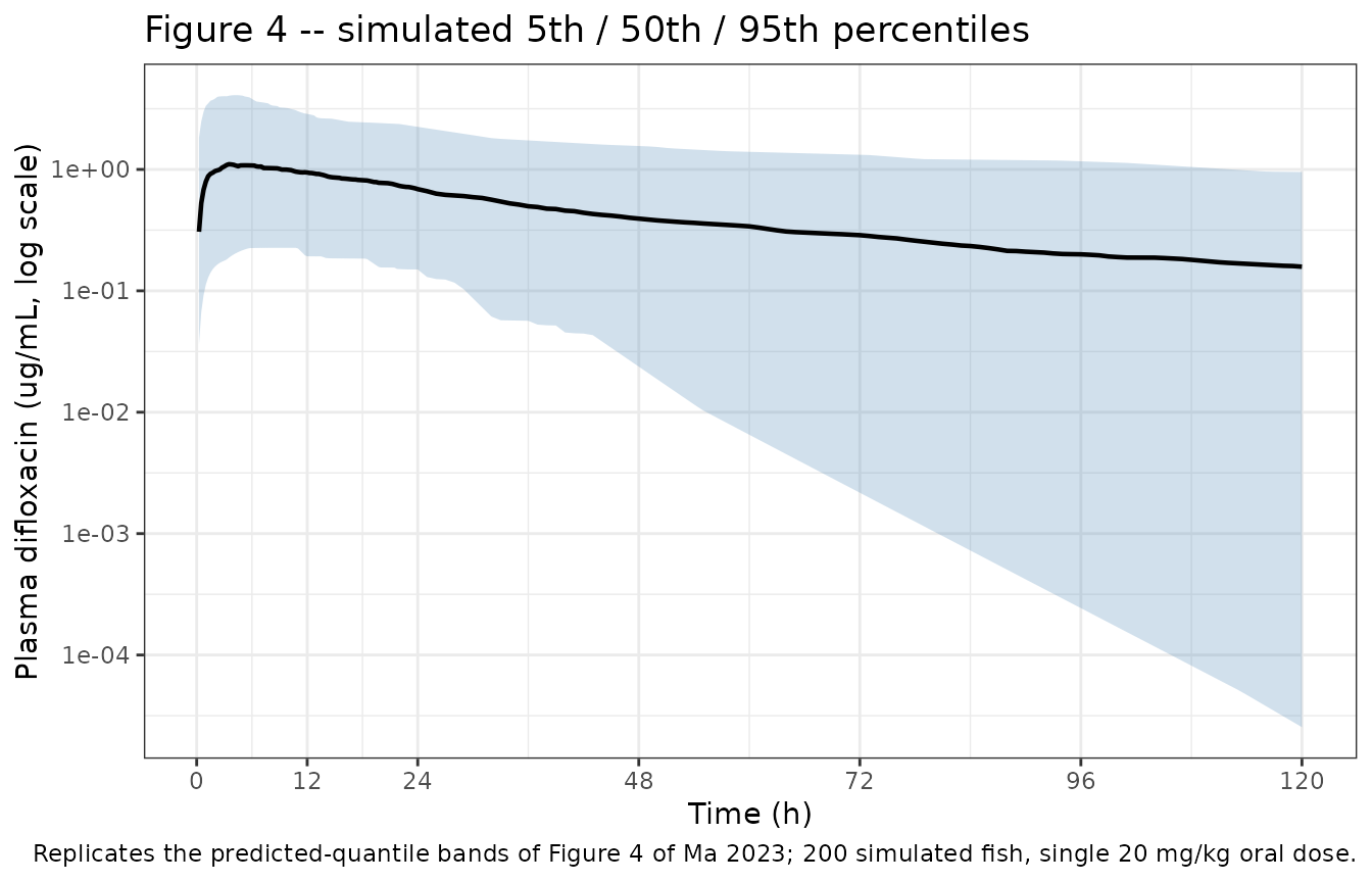
Ma 2023 Figure 4 is a VPC of the final model over 0 to 120 h with 1000 simulation replicates. The observed data are not published, so only the predicted quantiles can be reproduced. The paper describes the between-fish variability as “huge”, and the packaged omegas bear that out.
# rxSetSeed() fixes rxode2's stream per solver thread but NOT across thread
# counts, so a CI runner draws a different cohort than a workstation. Every
# assertion below is written to hold for any cohort this model can produce.
rxode2::rxSetSeed(20230627)

n_fish <- 200L  # cap is 200 per arm
grid_cohort <- sort(unique(c(
  seq(0, 24, by = 0.25), seq(25, 120, by = 1), seq(124, 480, by = 4)
)))
ev_cohort <- rxode2::et(amt = 20, cmt = "depot") |>
  rxode2::et(grid_cohort) |>
  rxode2::et(id = seq_len(n_fish))

sim_cohort <-
  rxode2::rxSolve(mod, ev_cohort, returnType = "data.frame") |>
  mutate(treatment = "20 mg/kg")
#> ℹ parameter labels from comments will be replaced by 'label()'

# The ODE integrator can undershoot zero by about its absolute tolerance;
# a genuinely negative concentration would be comparable to the peak.
stopifnot(
  dplyr::n_distinct(sim_cohort$id) == n_fish,
  all(sim_cohort$Cc >= -1e-6 * max(sim_cohort$Cc, na.rm = TRUE))
)
Gate 3 – the omega block reproduces as encoded
Per-fish ka, vc and cl are
returned directly by rxSolve, so the realised cohort can be
checked against the encoded log-normal parameters without any NCA
step.
per_fish <- sim_cohort |>
  group_by(id) |>
  summarise(ka = first(ka), vc = first(vc), cl = first(cl), .groups = "drop")

realised <- tibble::tibble(
  parameter = c("ka", "vc", "cl"),
  encoded_median = c(1.18, 14.18, 0.20),
  encoded_omega  = sqrt(c(0.69, 1.12, 0.98)),
  cohort_median  = c(median(per_fish$ka), median(per_fish$vc), median(per_fish$cl)),
  cohort_sd_log  = c(sd(log(per_fish$ka)), sd(log(per_fish$vc)), sd(log(per_fish$cl)))
) |>
  mutate(
    median_log_ratio = log(cohort_median / encoded_median),
    sd_diff          = cohort_sd_log - encoded_omega
  )

# These are COHORT statistics, so the bounds must survive any draw.
# Measured over the three parameters at 1 / 2 / 4 / 8 / 16 solver threads:
#   max |log median ratio| = 0.156 / 0.028 / 0.126 / 0.068 / 0.247
#   max |SD difference|    = 0.033 / 0.063 / 0.058 / 0.084 / 0.073
# Theory agrees: SE(log median) ~= 1.2533 * omega / sqrt(n) = 0.094 at
# worst (vc), and SE(SD) ~= omega / sqrt(2n) = 0.053 at worst. The bounds
# below sit at ~6 SE, outside the whole observed range, and still go red
# on a decimal-point or variance-vs-SD error, which shift these by 1 or
# more. Do not tighten them back onto a single observed run.
stopifnot(
  max(abs(realised$median_log_ratio)) < 0.60,
  max(abs(realised$sd_diff)) < 0.30
)

realised |>
  mutate(across(where(is.numeric), \(x) round(x, 3))) |>
  dplyr::rename(
    "Parameter" = parameter,
    "Encoded median" = encoded_median,
    "Encoded omega" = encoded_omega,
    "Cohort median" = cohort_median,
    "Cohort SD(log)" = cohort_sd_log,
    "log(median ratio)" = median_log_ratio,
    "SD difference" = sd_diff
  ) |>
knitr::kable(caption = "Gate 3: realised cohort vs the encoded log-normal IIV.")| Parameter | Encoded median | Encoded omega | Cohort median | Cohort SD(log) | log(median ratio) | SD difference |
|---|---|---|---|---|---|---|
| ka | 1.18 | 0.831 | 1.143 | 0.836 | -0.032 | 0.006 |
| vc | 14.18 | 1.058 | 16.572 | 1.028 | 0.156 | -0.030 |
| cl | 0.20 | 0.990 | 0.207 | 1.023 | 0.037 | 0.033 |
# The paper calls the between-fish variability "huge" (Discussion) and
# reports omega^2 above 0.9 for both V and CL. Gate 3 above checks the
# parameter columns; this checks that the variability actually propagates
# through the ODE solve and the residual-error draw into the simulated
# observations.
#
# The statistic is the INTERQUARTILE ratio, not a 5th/95th ratio. With
# omega^2 of 1.12 on V the far tail is extremely heavy and a P95/P05 ratio
# from 200 draws is useless as a gate: measured 61.3 / 15.0 / 19.0 / 18.6 /
# 89.8 at 1 / 2 / 4 / 8 / 16 solver threads, a six-fold swing on identical
# source. The IQR ratio over the same five runs was 3.08 / 3.21 / 3.19 /
# 2.80 / 3.55.
spread_24h <- sim_cohort |>
  filter(abs(time - 24) < 1e-8) |>
  summarise(ratio = quantile(sim, 0.75) / quantile(sim, 0.25)) |>
  pull(ratio)

# A bound of 2 sits below the whole observed 2.80-3.55 range and still goes
# red on the failure this gate exists to catch: with the etas dropped the
# only remaining spread is the residual error, giving an IQR ratio of
# exp(2 * 0.6745 * 0.16) = 1.24.
stopifnot(spread_24h > 2)
c(`P75:P25 ratio at 24 h` = round(spread_24h, 2))
#> P75:P25 ratio at 24 h
#>                  3.21
Gate 4 – the free AUC/MIC conclusion (Discussion)
The paper’s clinical conclusion is a short arithmetic chain built on the model-derived AUC0-inf, a literature plasma protein-binding estimate and literature MIC data. Running it from the model’s own AUC rather than the published 102.05 makes it an end-to-end check of the packaged model against a published conclusion.
# Discussion, final paragraph:
#  - plasma protein binding of difloxacin in healthy gibel carp is 52.66% to
#    80.56%; the authors assume the mean, 66.7%, for crucian carp
#  - MIC of difloxacin against Aeromonas hydrophila isolated from carps:
#    0.83 to 4 ug/mL
#  - fluoroquinolone efficacy target: free AUC/MIC >= 125
fu <- 1 - 0.667
mic_range <- c(0.83, 4)
target_fauc_mic <- 125

free_auc_model <- auc_sim * fu
ratios_model   <- free_auc_model / mic_range

published_chain <- c(free_auc = 33.98, ratio_mic4 = 8.495, ratio_mic083 = 40.93)
model_chain     <- c(free_auc = free_auc_model,
                     ratio_mic4 = ratios_model[2], ratio_mic083 = ratios_model[1])

# Deterministic (typical value); the only slack is the 2% tvCL rounding
# already characterised in Gate 1, which propagates linearly through the
# whole chain.
stopifnot(all(abs((model_chain - published_chain) / published_chain * 100) < 3))

# The qualitative conclusion must survive: neither end of the MIC range
# reaches the efficacy target at 20 mg/kg.
stopifnot(all(ratios_model < target_fauc_mic))

tibble::tibble(
  Quantity = c("Free AUC0-inf (h*ug/mL)",
               "Free AUC/MIC at MIC 4 ug/mL",
               "Free AUC/MIC at MIC 0.83 ug/mL"),
  `Ma 2023 Discussion` = published_chain,
  Model = round(model_chain, 3),
  `% diff` = round((model_chain - published_chain) / published_chain * 100, 2)
) |>
knitr::kable(caption = "Gate 4: the paper's free AUC/MIC chain, recomputed from the packaged model.")| Quantity | Ma 2023 Discussion | Model | % diff |
|---|---|---|---|
| Free AUC0-inf (h*ug/mL) | 33.980 | 33.300 | -2.00 |
| Free AUC/MIC at MIC 4 ug/mL | 8.495 | 8.325 | -2.00 |
| Free AUC/MIC at MIC 0.83 ug/mL | 40.930 | 40.120 | -1.98 |
Both ends of the reported MIC range fall well short of the free AUC/MIC target of 125, reproducing the paper’s conclusion that a single 20 mg/kg oral dose is insufficient against Aeromonas hydrophila in crucian carp. Inverting the target gives the highest MIC the dose could in principle cover:
mic_covered <- free_auc_model / target_fauc_mic
c(`max MIC covered at free AUC/MIC 125 (ug/mL)` = round(mic_covered, 3))
#> max MIC covered at free AUC/MIC 125 (ug/mL)
#>                                       0.266
0.27 ug/mL is below the lowest MIC (0.83 ug/mL) the authors cite, which is the substance of the abstract’s statement that the dose “cannot generate adequate plasma concentrations to inhibit pathogens with MIC values above 0.83 ug/mL”.
Assumptions and deviations
-
The omega off-diagonals are not published. Section
2.5 states that the final model used a full variance-covariance
matrix over
etaV,etaCLandetaKa– indeed that is the only structural difference between the basic and final models, and it is what drove the reported delta -2LL of 42.72. Table 3 publishes only the three diagonal variances; no covariance, correlation or full matrix appears anywhere in the paper or its figures. Rather than invent off-diagonal values, the packaged model leaves the three etas independent. Typical-value predictions (Gates 1, 2 and 4) are unaffected, because omega does not enter them. Cohort-level quantiles (the Figure 4 replication and Gate 3’s spread check) will be somewhat narrower or wider than the paper’s depending on the sign of the true correlations, most importantly theetaCL/etaVpair, which jointly determine the terminal slope. -
tvCLis encoded as the printed 0.20 L/h/kg. Table 4’s secondary parameters were computed from an unrounded 0.19598 L/h/kg (recovered above by inverting Equations 2 and 3). Using the printed 2-dp value costs a uniform 2.0% on AUC0-inf, T1/2 and every quantity derived from them. The printed value is used because it is what Table 3, the abstract, the results and the conclusions all state; the arithmetic to recover the unrounded value is shown in the “rounding-interval” chunk for anyone who prefers it. -
stdev0is treated as a log-scale SD, not a concentration. Justified in the “residual error model” section above from Section 2.5’s explicit “log-additive error model”. - Table 2’s CL is a typo. Demonstrated numerically above. No model parameter depends on Table 2.
-
Body weight is recorded but unused. It is
registered under
covariatesDataExcluded, notcovariateData, because Ma 2023 screened it and rejected it (delta -2LL = 3.02 against a 6.64 threshold). Note that weight scaling is nevertheless implicit in the units: the dose is mg/kg and V/F and CL/F are per kg, so the rejected test was for a departure from strict proportionality, not for the absence of any weight effect. Simulations must therefore supplyamtin mg/kg body weight, andCccomes back in ug/mL without any further scaling. - Observed data are not reproduced. Ma 2023 publishes no concentration table, so Figures 1 to 4 cannot be overlaid with observations; only the model-side quantities are reproduced here. Table 1’s design and body weights are transcribed exactly and are the only individual-level data in the paper.
- Single temperature. All parameters apply at 21.3 +/- 1.2 degC. The Discussion documents a roughly two-fold change in difloxacin half-life in crucian carp between 10 and 20 degC, so these values must not be extrapolated to other rearing temperatures.
-
No non-paper-derived parameter values. Every
ini()entry is transcribed from Ma 2023 Table 3; nothing was digitised from a figure, obtained by correspondence or carried from an upstream model.