Rivaroxaban pediatric (Willmann 2021)
Source:vignettes/articles/Willmann_2021_rivaroxaban.Rmd
Willmann_2021_rivaroxaban.RmdModel and source
- Citation: Willmann S, Coboeken K, Zhang Y, Mayer H, Ince I, Mesic E, Thelen K, Kubitza D, Lensing AWA, Yang H, Zhu P, Mueck W, Drenth HJ, Lippert J. Population pharmacokinetic analysis of rivaroxaban in children and comparison to prospective physiologically-based pharmacokinetic predictions. CPT Pharmacometrics Syst Pharmacol. 2021;10(10):1195-1207. doi:10.1002/psp4.12688
- Description: Pediatric population PK model for rivaroxaban developed on the integrated EINSTEIN-Jr phase I / I-II / II / III dataset and interim PK from part A of the UNIVERSE study (524 children, 1988 plasma concentrations, age birth to <18 years, body weight 2.7-194 kg). Two-compartment disposition with first-order absorption and first-order elimination from the central compartment. Body weight enters as estimated allometric scaling on CL, Q, Vc, and Vp, centred on the 82.48 kg median of the integrated adult popPK analysis (a shared exponent is used for Vc and Vp). The undiluted ready-to-use oral suspension has a lower first-order absorption rate constant ka than the other three formulations (tablet, granules for oral suspension, and diluted ready-to-use oral suspension), which share a common ka. Relative oral bioavailability decreases with dose per body weight following an exponential function carried over from the integrated adult popPK analysis (anchored to F1 = 1 at 10 mg / 82.48 kg = 0.1213 mg/kg). Inter-individual variability is on CL and F1 only (no IIV on Ka, Vc, Vp, or Q); residual error is proportional. Age, eGFR (Schwartz and Rhodin), serum creatinine, comedications (CYP3A4 inhibitors / inducers, P-gp inhibitors), and Fontan status were tested and not retained.
- Article: https://doi.org/10.1002/psp4.12688
Population
The integrated pediatric popPK analysis pooled 1988 rivaroxaban plasma concentrations from 524 children (47.1% female) across the EINSTEIN-Jr phase I, I-II, II, and III studies for acute venous thromboembolism and the UNIVERSE phase III part A study in post-Fontan children with congenital heart disease (Willmann 2021 Table 1; supplement Table S1). Body weight spanned 2.7-194 kg (median 29.5) and age birth to less than 18 years (median 9.0). Eighty-six subjects (16.4%) were younger than two years. Bodyweight-adjusted doses ranged 0.4-20 mg per administration with once-daily, twice-daily, or thrice-daily regimens stratified by weight band (Willmann 2021 Discussion p. 1201: o.d. for body weight >=30 kg, b.i.d. for 12-<30 kg, t.i.d. for <12 kg).
Programmatic metadata:
rxode2::rxode(readModelDb("Willmann_2021_rivaroxaban"))$population.
Source trace
Every parameter’s in-file source-trace comment in
inst/modeldb/specificDrugs/Willmann_2021_rivaroxaban.R is
reproduced here for one-place auditing.
| Element | Value (with units) | Source location |
|---|---|---|
| ka (tablets, granules, diluted suspension) | 0.799 1/h | Willmann 2021 Table 2 |
| ka (undiluted ready-to-use oral suspension) | 0.226 1/h | Willmann 2021 Table 2 |
| CL at 82.48 kg | 8.02 L/h | Willmann 2021 Table 2 |
| Vc at 82.48 kg | 53.2 L | Willmann 2021 Table 2 |
| Vp at 82.48 kg | 59.1 L | Willmann 2021 Table 2 |
| Q at 82.48 kg | 2.50 L/h | Willmann 2021 Table 2 |
| Allometric WT exponent on CL | 0.481 | Willmann 2021 Table 2 (estimated) |
| Allometric WT exponent on Vc and Vp (shared) | 0.821 | Willmann 2021 Table 2 (estimated) |
| Allometric WT exponent on Q | 0.761 | Willmann 2021 Table 2 (estimated) |
| F1MAX (upper asymptote of F1 vs DW) | 1.25 (fixed, a priori) | Willmann 2021 supplement S2 NONMEM $PK |
| F1MIN (lower asymptote of F1 vs DW) | 0.59 (fixed, a priori) | Willmann 2021 supplement S2 NONMEM $PK |
| D50 (half-decline dose per WT) | 14.4/82.48 mg/kg (fixed) | Willmann 2021 supplement S2 NONMEM $PK |
| omega^2 on CL | 0.0705 | Willmann 2021 Table 2 (footnote g: CV 27.0%) |
| omega^2 on F1 | 0.0612 | Willmann 2021 Table 2 (footnote g: CV 25.1%) |
| sigma^2 proportional residual | 0.220 (propSd = 0.4690) | Willmann 2021 Table 2 (footnote h: 46.9%) |
| 2-compartment ODE structure | n/a | Willmann 2021 Methods p. 1196; supplement S2 ADVAN4 TRANS4 |
| F1 = TF1 * exp(eta), TF1 = F1MIN + … | n/a | Willmann 2021 supplement S2 NONMEM $PK block (a priori from reference 19) |
Replicate Figure 2: relative oral bioavailability vs dose per body weight
The dose-dependent relative oral bioavailability function in the model is hard-coded a priori from the integrated adult popPK analysis (Willmann 2021 reference 19) after re-anchoring to F1 = 1.0 at 10 mg / 82.48 kg = 0.1213 mg/kg. We reproduce it algebraically (Figure 2 of the paper).
f1max <- 1.25
f1min <- 0.59
d50   <- 14.4 / 82.48

dw_grid <- seq(0.05, 0.6, length.out = 200)
f1_grid <- f1min + (f1max - f1min) * exp(-log(2) / d50 * dw_grid)

f1_df <- data.frame(dw = dw_grid, f1 = f1_grid)

anchor_points <- data.frame(
  dw    = c(0.1213, 0.30, 0.50),
  f1    = c(1.000,  0.791, 0.681),
  label = c("0.12 mg/kg (10 mg/82.48 kg)", "0.30 mg/kg", "0.50 mg/kg")
)

ggplot(f1_df, aes(dw, f1)) +
  geom_line(colour = "red", linewidth = 1) +
  geom_point(data = anchor_points, aes(dw, f1), size = 3) +
  geom_text(data = anchor_points, aes(dw, f1, label = label),
            hjust = -0.05, vjust = 1.5, size = 3) +
  scale_x_continuous(breaks = seq(0, 0.6, 0.1), limits = c(0, 0.6)) +
  scale_y_continuous(breaks = seq(0.5, 1.3, 0.1), limits = c(0.55, 1.30)) +
  labs(
    x = "Dose per body weight (mg/kg)",
    y = "Relative oral bioavailability F1 (unitless)",
    title = "Relative oral bioavailability vs dose per body weight",
    caption = paste(
      "Replicates Figure 2 of Willmann 2021. Anchor points (Results p. 1199):",
      "F1 = 1.000 at 0.12 mg/kg, 0.791 at 0.30 mg/kg, 0.681 at 0.50 mg/kg."
    )
  ) +
  theme_minimal()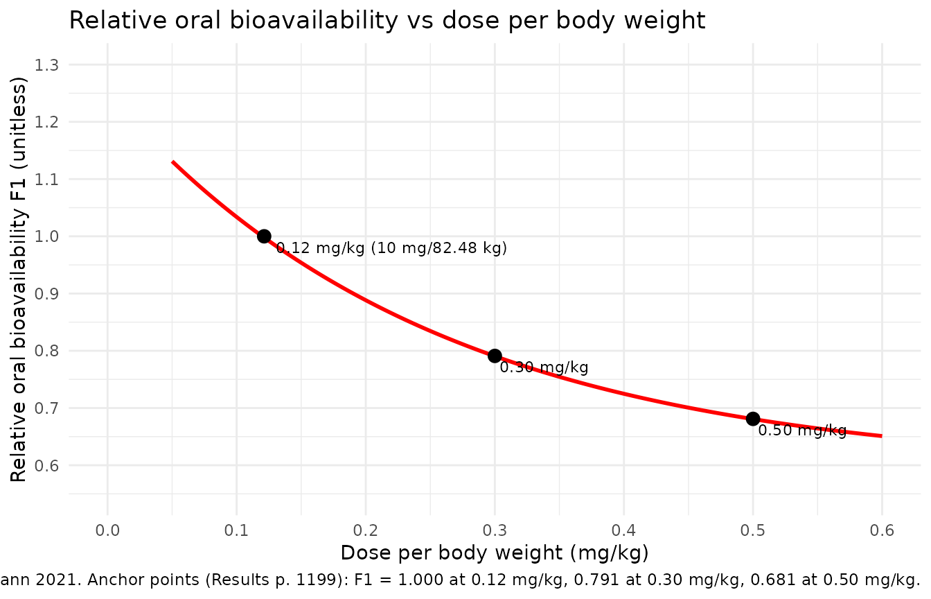
Replicate Figure 3: clearance vs body weight (typical-value)
The model’s typical-value clearance follows the allometric form
cl = 8.02 * (WT/82.48)^0.481. The paper’s Figure 3 plots
individual post-hoc CL estimates against age; here we draw the
typical-value curve versus body weight (which is the model’s actual
covariate; age is not retained as a CL covariate in the final
model).
wt_grid <- exp(seq(log(2.5), log(200), length.out = 200))
cl_typ <- 8.02 * (wt_grid / 82.48)^0.481

cl_df <- data.frame(WT = wt_grid, cl = cl_typ)

ggplot(cl_df, aes(WT, cl)) +
  geom_line(linewidth = 1) +
  scale_x_log10(breaks = c(2.5, 5, 10, 20, 50, 100, 200)) +
  scale_y_log10(breaks = c(0.5, 1, 2, 5, 10, 20)) +
  labs(
    x = "Body weight (kg)",
    y = "Typical-value CL (L/h)",
    title = "Typical-value rivaroxaban clearance vs body weight",
    caption = paste(
      "Underlies Figure 3 of Willmann 2021 (which plots CL vs age).",
      "CL is allometrically scaled on WT (exponent 0.481, reference 82.48 kg);",
      "age is not retained as a CL covariate in the final model."
    )
  ) +
  theme_minimal()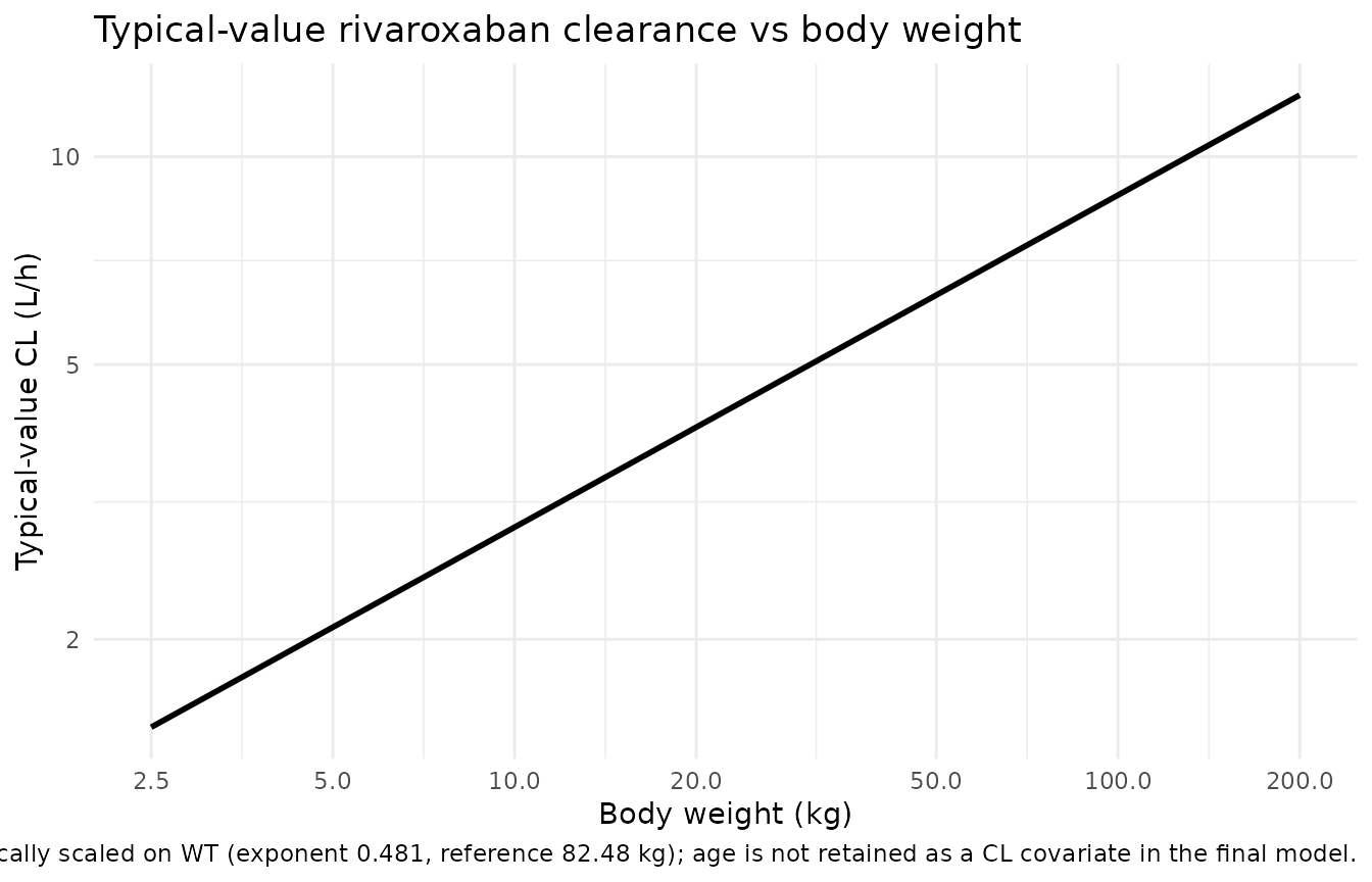
Virtual cohort for steady-state simulation
We build a pooled multi-cohort event table that mirrors the
EINSTEIN-Jr phase III by-age-group dosing scheme used by Willmann 2021
to compute the steady-state exposure metrics in supplement Table S2.
Each cohort uses the cohort mean body weight (supplement Table S1) and a
representative phase-III bodyweight-banded daily dose split across the
regimen (o.d., b.i.d., or t.i.d.) appropriate for the weight band
(Willmann 2021 Discussion p. 1201). Doses are administered as the tablet
/ granule / diluted formulation
(FORM_UNDILUTED_SUSP = 0).
set.seed(20210710L)

make_cohort <- function(age_group, n, wt_kg, total_daily_mg, regimen,
                        id_offset, days = 14) {
  per_dose_mg <- total_daily_mg / regimen
  tau_h <- 24 / regimen
  dose_times <- seq(0, days * 24 - tau_h, by = tau_h)
  obs_times <- sort(unique(c(
    dose_times,
    seq(0, days * 24, by = 1)
  )))

  ids <- id_offset + seq_len(n)

  dose_rows <- tidyr::expand_grid(id = ids, time = dose_times) |>
    dplyr::mutate(
      amt  = per_dose_mg,
      evid = 1L,
      cmt  = "depot"
    )
  obs_rows <- tidyr::expand_grid(id = ids, time = obs_times) |>
    dplyr::mutate(
      amt  = NA_real_,
      evid = 0L,
      cmt  = "central"
    )

  events <- dplyr::bind_rows(dose_rows, obs_rows) |>
    dplyr::arrange(id, time, dplyr::desc(evid)) |>
    dplyr::mutate(
      age_group           = age_group,
      regimen             = regimen,
      total_daily_mg      = total_daily_mg,
      per_dose_mg         = per_dose_mg,
      WT                  = wt_kg,
      FORM_UNDILUTED_SUSP = 0L,
      DOSE_RIV_MGKG       = per_dose_mg / wt_kg
    )

  events
}

cohorts <- dplyr::bind_rows(
  make_cohort(age_group = "12 to <18 years",     n = 30, wt_kg = 67.9,
              total_daily_mg = 20.0, regimen = 1L, id_offset =   0L),
  make_cohort(age_group = "6 to <12 years",      n = 30, wt_kg = 32.4,
              total_daily_mg = 20.0, regimen = 1L, id_offset = 100L),
  make_cohort(age_group = "2 to <6 years",       n = 30, wt_kg = 16.4,
              total_daily_mg = 12.0, regimen = 2L, id_offset = 200L),
  make_cohort(age_group = "6 months to <2 years",n = 30, wt_kg =  9.49,
              total_daily_mg =  9.0, regimen = 3L, id_offset = 300L),
  make_cohort(age_group = "birth to <6 months",  n = 30, wt_kg =  4.05,
              total_daily_mg =  6.0, regimen = 3L, id_offset = 400L)
)

stopifnot(!anyDuplicated(unique(cohorts[, c("id", "time", "evid")])))
Simulate steady-state PK
mod <- rxode2::rxode(nlmixr2lib::readModelDb("Willmann_2021_rivaroxaban"))

sim <- rxode2::rxSolve(
  mod,
  events = cohorts,
  keep = c("age_group", "regimen", "total_daily_mg", "per_dose_mg",
           "WT", "FORM_UNDILUTED_SUSP", "DOSE_RIV_MGKG")
) |>
  as.data.frame()

# Convert plasma concentration mg/L -> ug/L to match the paper's reporting units.
sim$Cc_ugL <- sim$Cc * 1000
Steady-state interval (day 13 to day 14)
The paper’s supplement Table S2 reports steady-state AUC(0-24)ss, Cmax,ss, and Ctrough,ss. We extract the day-13 to day-14 dosing window (the model has reached effective steady state for clearance-driven exposure by that point) and compute PKNCA-based exposure metrics.
tau <- 24

# Restrict to the final 24 h window for steady-state NCA.
ss_window <- sim |>
  dplyr::filter(time >= (14 - 1) * 24, time <= 14 * 24) |>
  dplyr::mutate(time_ss = time - (14 - 1) * 24)

sim_nca <- ss_window |>
  dplyr::filter(!is.na(Cc)) |>
  dplyr::select(id, time_ss, Cc = Cc_ugL, age_group)

# Defensive time-zero guarantee: if the per-id grid did not produce a
# time_ss = 0 row, add one with Cc = trough (the value at the start of
# the interval).
trough_rows <- sim_nca |>
  dplyr::group_by(id, age_group) |>
  dplyr::slice_min(time_ss, n = 1, with_ties = FALSE) |>
  dplyr::ungroup() |>
  dplyr::mutate(time_ss = 0)

sim_nca <- dplyr::bind_rows(sim_nca, trough_rows) |>
  dplyr::distinct(id, age_group, time_ss, .keep_all = TRUE) |>
  dplyr::arrange(id, age_group, time_ss)

dose_df <- cohorts |>
  dplyr::filter(evid == 1L, time >= (14 - 1) * 24, time < 14 * 24) |>
  dplyr::mutate(time_ss = time - (14 - 1) * 24) |>
  dplyr::select(id, time_ss, amt, age_group)

conc_obj <- PKNCA::PKNCAconc(sim_nca, Cc ~ time_ss | age_group + id)
dose_obj <- PKNCA::PKNCAdose(dose_df, amt ~ time_ss | age_group + id)

intervals <- data.frame(
  start    = 0,
  end      = tau,
  cmax     = TRUE,
  tmax     = TRUE,
  cmin     = TRUE,
  auclast  = TRUE
)

nca_res <- PKNCA::pk.nca(PKNCA::PKNCAdata(conc_obj, dose_obj,
                                          intervals = intervals))

nca_summary <- as.data.frame(nca_res$result) |>
  dplyr::filter(PPTESTCD %in% c("cmax", "cmin", "auclast")) |>
  dplyr::group_by(age_group, PPTESTCD) |>
  dplyr::summarise(value = exp(mean(log(PPORRES[PPORRES > 0]))),
                   .groups = "drop") |>
  tidyr::pivot_wider(names_from = PPTESTCD, values_from = value)

knitr::kable(
  nca_summary,
  digits = c(NA, 0, 1, 0),
  caption = paste(
    "Simulated steady-state NCA (geometric mean across cohort subjects)",
    "for the day 13-14 dosing window, by age group."
  ),
  col.names = c("Age group", "AUC0-tau (ug*h/L)", "Cmin,ss (ug/L)",
                "Cmax,ss (ug/L)")
)| Age group | AUC0-tau (ug*h/L) | Cmin,ss (ug/L) | Cmax,ss (ug/L) |
|---|---|---|---|
| 12 to <18 years | 2302 | 237.7 | 26 |
| 2 to <6 years | 2430 | 198.3 | 30 |
| 6 months to <2 years | 2397 | 161.6 | 38 |
| 6 to <12 years | 2454 | 327.3 | 18 |
| birth to <6 months | 2316 | 171.4 | 29 |
Comparison against published Table S2 popPK exposure metrics
Willmann 2021 supplement Table S2 reports geometric-mean AUC(0-24)ss, Cmax,ss, and Ctrough,ss in each age group, derived from individual post-hoc PopPK predictions of the EINSTEIN-Jr phase III study subjects. The simulated typical-cohort exposures below should fall within the same order of magnitude; per-age-group discrepancy reflects (a) the allometric scaling underprediction of clearance for children under 2 years (Willmann 2021 Discussion p. 1201) and (b) cohort heterogeneity that this typical-value cohort does not capture.
published <- tibble::tribble(
  ~age_group,               ~auc_pop,  ~cmax_pop,  ~ctrough_pop,
  "12 to <18 years",         2120,      237,        20.7,
  "6 to <12 years",          1960,      184,        21.4,
  "2 to <6 years",           2380,      182,        31.6,
  "6 months to <2 years",    1740,      129,        21.2,
  "birth to <6 months",      1740,      129,        21.2
)

cmp <- dplyr::left_join(nca_summary, published, by = "age_group") |>
  dplyr::transmute(
    `Age group`              = age_group,
    `AUC0-tau (sim, ug*h/L)` = round(auclast, 0),
    `AUC0-tau (paper)`       = auc_pop,
    `Cmax,ss (sim, ug/L)`    = round(cmax, 0),
    `Cmax,ss (paper)`        = cmax_pop,
    `Ctrough,ss (sim, ug/L)` = round(cmin, 1),
    `Ctrough,ss (paper)`     = ctrough_pop
  )

knitr::kable(
  cmp,
  caption = paste(
    "Simulated vs. published popPK-derived steady-state NCA",
    "(Willmann 2021 supplement Table S2; the paper pools the birth-<6 mo and",
    "6 mo-<2 yr groups into a single birth-<2 yr stratum, so both cohorts",
    "compare against the same Table S2 row)."
  )
)| Age group | AUC0-tau (sim, ug*h/L) | AUC0-tau (paper) | Cmax,ss (sim, ug/L) | Cmax,ss (paper) | Ctrough,ss (sim, ug/L) | Ctrough,ss (paper) |
|---|---|---|---|---|---|---|
| 12 to <18 years | 2302 | 2120 | 238 | 237 | 26.4 | 20.7 |
| 2 to <6 years | 2430 | 2380 | 198 | 182 | 29.5 | 31.6 |
| 6 months to <2 years | 2397 | 1740 | 162 | 129 | 38.2 | 21.2 |
| 6 to <12 years | 2454 | 1960 | 327 | 184 | 18.2 | 21.4 |
| birth to <6 months | 2316 | 1740 | 171 | 129 | 28.6 | 21.2 |
Assumptions and deviations
- Representative per-age-group cohort. The vignette uses a single representative body weight (cohort mean from supplement Table S1) and a single representative phase-III bodyweight-banded daily dose per age group; the actual EINSTEIN-Jr phase III cohort spans a wider weight range and individual dose per body weight varies across weight bands. The supplementary Table S2 figures pool over the full per-subject weight / dose variability, so per-cohort discrepancy is expected.
-
No upstream / downstream cohort-mixing. Each cohort
uses disjoint IDs via
id_offset(Robbie 2012 / Clegg 2024 pattern); duplicate IDs across cohorts would silently merge into Frankenstein subjects inrxSolve. - Race / ethnicity not modelled. No effect of Japanese, Chinese, or Asian (outside Japan and China) origin was retained in the final model (Willmann 2021 Results p. 1199 and supplementary Figures S7-S9); the cohort does not stratify on race.
- Age not retained as a CL covariate. Willmann 2021 Results p. 1199: “No effect of age on CL or F1 could be identified by the model.” The population CL is allometrically scaled on weight only. The paper’s Figure 3 shows that the popPK model underpredicts clearance in children below 2 years of age relative to individual EBE estimates, but this is a known limitation and is not captured by the structural model.
-
Renal function, comedication, and Fontan status not
retained. Four measures of renal function (eGFR Schwartz, eGFR
Rhodin, serum creatinine ratio to ULN, categorical creatinine score),
three CYP3A4 comedication indicators (weak inhibitor, moderate
inhibitor, inducer), P-gp inhibitor, and Fontan status were tested. None
were retained in the final model (Willmann 2021 Results p. 1199). These
are documented in
covariatesDataExcludedof the model file metadata for provenance but are not used in the structural model. - Steady-state day choice. The simulation runs 14 days of dosing and extracts the day-13 to day-14 dosing window for NCA; with a typical rivaroxaban terminal half-life around 4-12 h depending on weight, steady state is comfortably reached by then.
-
F1 anchoring. The
f1max,f1min, andd50constants are reproduced verbatim from the supplement S2 NONMEM$PKblock. They are not estimated by the pediatric fit (held as a priori constants carried over from the integrated adult popPK analysis in Willmann 2021 reference 19).