Cis-, trans- and total cefprozil (Jang 2019) • nlmixr2lib

Model and source

Jang 2019 is the first published population PK analysis of cefprozil. Cefprozil is marketed as a roughly 9:1 mixture of its cis- and trans-isomers, which differ in antimicrobial potency (cis is about six-fold more active against Gram-negative organisms), so the authors fitted three independent models – one to the cis concentrations, one to the trans concentrations, and one to their sum. All three are packaged separately, exactly as the authors built them.

modelNames <- c(
  cis = "Jang_2019_cefprozil_cis",
  trans = "Jang_2019_cefprozil_trans",
  total = "Jang_2019_cefprozil_total"
)
uis <- lapply(modelNames, function(nm) rxode2::rxode(readModelDb(nm)))
#> ℹ parameter labels from comments will be replaced by 'label()'
#> ℹ parameter labels from comments will be replaced by 'label()'
#> ℹ parameter labels from comments will be replaced by 'label()'

Citation: Jang JH, Jeong SH, Cho HY, Lee YB. (2019). Population Pharmacokinetics of Cis-, Trans-, and Total Cefprozil in Healthy Male Koreans. Pharmaceutics 11(10):531. doi:10.3390/pharmaceutics11100531.
Article: https://doi.org/10.3390/pharmaceutics11100531

Each analyte is a one-compartment model with first-order absorption, an absorption lag time and first-order elimination. The three differ in three ways, all of which the packaged models preserve:

The three Jang 2019 models differ in covariate model, in which parameters carry IIV, and in residual-error form. Note that the trans model is the mirror image of the other two: IIV on Ka but none on V.
Analyte	Covariate on CL	IIV terms	Residual error
cis	CrCl (linear, centred)	V, CL, Tlag	log-additive (lnorm)
trans	none retained	Ka, CL, Tlag	proportional
total	CrCl (linear, centred)	V, CL, Tlag	log-additive (lnorm)

Population

Thirty-five healthy Korean men from the reference arm of a two-way crossover bioequivalence study (Bioequivalence Test No. 611) each received a single 1000 mg oral dose of cefprozil after an overnight fast, with 12 plasma samples collected over 12 h (420 samples per analyte). The cohort is young (21–27 years, median 24), of normal build (53.1–91.8 kg, median 69.5) and has normal-to-supranormal renal function (CrCl 86.57–159.05 mL/min, median 124.41, Cockcroft-Gault). Cefprozil isomers were assayed separately by UPLC-ESI-MS/MS with LLOQs of 5 ng/mL (cis) and 15 ng/mL (trans); total cefprozil is their arithmetic sum. Baseline demographics are Jang 2019 Table 1.

Because the cohort spans a narrow band of supranormal renal function, the creatinine-clearance effect below is informed only over roughly 87–159 mL/min; Jang 2019’s Discussion makes the same caveat when it proposes the model for renal dose adjustment.

The same information is available programmatically via rxode2::rxode(readModelDb("Jang_2019_cefprozil_total"))$population.

Source trace

Every ini() entry carries an in-file comment naming its source location. They are collected here for review. Volumes and clearances are printed by Jang 2019 in mL and mL/h and are divided by 1000 in the model files so that a dose in mg yields mg/L = ug/mL, the unit the paper reports concentrations in.

Parameter	cis	trans	total	Source location
`lka` (Ka, 1/h)	0.429	0.829	0.432	Table 4, per-analyte Final model, `tvKa`
`lvc` (V/F, mL)	14,308.10	34,617.50	14,713.10	Table 4, per-analyte Final model, `tvV`
`lcl` (CL/F, mL/h)	17,150.70	17,701.80	17,226.20	Table 4, per-analyte Final model, `tvCl`
`ltlag` (Tlag, h)	0.352	0.352	0.351	Table 4, per-analyte Final model, `tvTlag`
`e_crcl_cl` (per mL/min)	3.04e-3	n/a	2.87e-3	Table 5, `dCldCrCl` (Table 4 rounds both to 0.003)
`etalvc` (omega^2 V)	0.127	n/a	0.124	Table 4, per-analyte Final model
`etalcl` (omega^2 CL)	0.016	0.017	0.016	Table 4, per-analyte Final model
`etaltlag` (omega^2 Tlag)	0.021	0.094	0.021	Table 4, per-analyte Final model
`etalka` (omega^2 Ka)	n/a	0.076	n/a	Table 4, Trans-cefprozil Final model
`expSd` / `propSd` (sigma)	0.193	0.232	0.189	Table 4, per-analyte Final model
CL covariate equation	`Cl = Cltv * (1 + (CrCl - 124.41) * dCldCrCl) * exp(etaCl)`	n/a	same as cis	Final-model equations, p. 7
Centring constant (mL/min)	124.41	n/a	124.41	Table 1, median CrCl
Structure	one-compartment, first-order absorption + lag	same	same	Results 3.3, Conclusions

Two source-trace notes:

The dCldCrCl coefficient is printed twice. Table 4 rounds it to 0.003 for both analytes; Table 5 prints the same final-model estimate to three significant figures as 3.04e-3 (cis) and 2.87e-3 (total). The models use the Table 5 values as the more precise rendering of one number.
The covariate enters linearly and centred, not on a log or power scale. The final-model equations on p. 7 are explicit about this, and the form matters: at the cohort extremes the multiplier spans only about 0.89–1.11.

Dose basis: which dose each model expects

Jang 2019 never states the dose amount entered into each analyte’s dataset. Every subject swallowed one 1000 mg cefprozil tablet, but the cis model was fitted to cis concentrations, so its CL/F is on a cis-mass basis. Getting this wrong is not a rounding error – it is a nine-fold error on the trans model – so it is derived here rather than assumed.

The derivation uses ratios of the paper’s own numbers, which is what makes it trustworthy: since AUC = Dose / CL for all three models, the ratio of two analytes’ doses is fixed by the ratio of their reported NCA AUCs and the ratio of their fitted clearances, and any systematic model-vs-NCA bias common to the three cancels out.

# Jang 2019 Discussion (p. 13), the paper's own noncompartmental results.
ncaPaper <- tibble::tribble(
  ~analyte, ~cmax, ~tmax, ~aucinf, ~halflife,
  "cis", 15.0, 1.96, 59.6, 1.67,
  "trans", 1.63, 1.96, 6.38, 1.50,
  "total", 16.6, 2.11, 66.0, 1.66
)

# Fitted CL/F (L/h) read back out of the packaged models.
clFitted <- vapply(uis, function(u) exp(u$theta[["lcl"]]), numeric(1))

# Dose of each isomer RELATIVE to the 1000 mg total, from ratios alone.
doseRel <- (ncaPaper$aucinf / ncaPaper$aucinf[ncaPaper$analyte == "total"]) *
  (clFitted[ncaPaper$analyte] / clFitted[["total"]])
doseImplied <- 1000 * doseRel

tibble::tibble(
  Analyte = ncaPaper$analyte,
  `Implied dose (mg)` = round(doseImplied, 1),
  `Rounded basis (mg)` = c(900, 100, 1000)
) |>
  knitr::kable(
    caption = "Dose basis implied by (AUC ratio) x (CL ratio) against the 1000 mg total, versus the round 9:1 isomer split the paper's Introduction quotes."
  )

Dose basis implied by (AUC ratio) x (CL ratio) against the 1000 mg total, versus the round 9:1 isomer split the paper’s Introduction quotes.
Analyte	Implied dose (mg)	Rounded basis (mg)
cis	899.1	900
trans	99.3	100
total	1000.0	1000

# Deterministic: pure arithmetic on published constants, so a tight bound is
# correct here (no simulation, no RNG). The implied split must land on the
# 900 / 100 / 1000 mg reading to within 1%.
doseBasis <- c(cis = 900, trans = 100, total = 1000)
stopifnot(
  max(abs(doseImplied / doseBasis[ncaPaper$analyte] - 1)) < 0.01,
  # And the isomer ratio must reproduce the "about 9:1" of the Introduction.
  abs(doseImplied[1] / doseImplied[2] - 9) < 0.5
)

The implied split is 899 mg / 99 mg / 1000 mg – a cis:trans ratio of 9.05:1, matching the “about 9:1” the Introduction quotes, and landing on the round 900 / 100 / 1000 mg reading to within 1%. The competing reading, that all three datasets carried the full 1000 mg, is decisively falsified: it would put the trans model’s AUC at 56.5 ugh/mL against the 6.38 ugh/mL the paper reports, a nine-fold error.

So: dose Jang_2019_cefprozil_cis with the cis content of the tablet (900 mg of a 1000 mg dose), Jang_2019_cefprozil_trans with the trans content (100 mg), and Jang_2019_cefprozil_total with the whole 1000 mg.

Virtual cohort

The individual data are not public. The cohort below reproduces Table 1’s creatinine-clearance distribution – the only covariate any of the three final models uses – as a truncated normal matched to the reported mean, SD and range. Each analyte is simulated as its own arm of 200 subjects on the paper’s actual sampling schedule plus a dense grid for plotting.

# set.seed() seeds R's RNG, not rxode2's; rxode2 partitions its streams per
# solver thread, so this cohort is reproducible here and different on a machine
# with a different thread count. Every assertion below is written to hold for
# any cohort these models can produce.
set.seed(20191014)

nPerArm <- 200L

# Jang 2019 Table 1: CrCl mean 124.55, SD 17.78, range 86.57-159.05 mL/min.
rtruncnorm <- function(n, mean, sd, lower, upper) {
  out <- numeric(0)
  while (length(out) < n) {
    draw <- stats::rnorm(2 * n, mean, sd)
    out <- c(out, draw[draw >= lower & draw <= upper])
  }
  out[seq_len(n)]
}

paperTimes <- c(0, 0.5, 0.75, 1, 1.25, 1.5, 1.75, 2, 3, 4, 8, 12)
denseTimes <- sort(unique(c(paperTimes, seq(0, 12, by = 0.05))))

makeArm <- function(analyte, dose, idOffset) {
  subj <- tibble::tibble(
    id = idOffset + seq_len(nPerArm),
    CRCL = rtruncnorm(nPerArm, 124.55, 17.78, 86.57, 159.05),
    analyte = analyte
  )
  doses <- subj |>
    dplyr::mutate(time = 0, amt = dose, evid = 1L, cmt = "depot")
  # Observation rows name the ODE STATE (central), never the algebraic
  # observable Cc -- naming Cc would auto-inject a cmt() slot and renumber
  # the compartments.
  obs <- subj |>
    tidyr::crossing(time = denseTimes) |>
    dplyr::mutate(amt = NA_real_, evid = 0L, cmt = "central")
  dplyr::bind_rows(doses, obs) |>
    dplyr::arrange(id, time, dplyr::desc(evid))
}

events <- dplyr::bind_rows(
  makeArm("cis", doseBasis[["cis"]], 0L),
  makeArm("trans", doseBasis[["trans"]], 1000L),
  makeArm("total", doseBasis[["total"]], 2000L)
)

# Disjoint IDs across arms: duplicate IDs silently merge into one subject.
stopifnot(!anyDuplicated(unique(events[, c("id", "time", "evid")])))

Simulation

Each analyte is solved with its own model; the arms are simulated separately because each model has a different parameter vector, then stacked for plotting.

simOne <- function(analyte) {
  # Base subsetting: `analyte` is both a column name and this function's
  # argument, so NSE here would be ambiguous.
  ev <- events[events$analyte == analyte, , drop = FALSE]
  rxode2::rxSolve(
    readModelDb(modelNames[[analyte]]),
    events = as.data.frame(ev),
    keep = c("CRCL", "analyte"),
    returnType = "data.frame"
  )
}
sim <- dplyr::bind_rows(lapply(names(modelNames), simOne))
#> ℹ parameter labels from comments will be replaced by 'label()'
#> ℹ parameter labels from comments will be replaced by 'label()'
#> ℹ parameter labels from comments will be replaced by 'label()'
sim$analyte <- factor(sim$analyte, levels = c("cis", "trans", "total"))
stopifnot(all(is.finite(sim$Cc)), all(sim$Cc >= 0))

Deterministic check: the ODE reproduces the closed form

Before comparing with the paper, confirm that each packaged model integrates to the analytical one-compartment oral solution with lag. Both sides use the same typical-value parameters, so the only difference is solver error and a tight bound is the right gate.

closedForm <- function(ui, dose, t) {
  ka <- exp(ui$theta[["lka"]])
  vc <- exp(ui$theta[["lvc"]])
  cl <- exp(ui$theta[["lcl"]])
  tl <- exp(ui$theta[["ltlag"]])
  kel <- cl / vc
  td <- pmax(t - tl, 0)
  (dose / vc) * (ka / (ka - kel)) * (exp(-kel * td) - exp(-ka * td))
}

cfCheck <- lapply(names(modelNames), function(a) {
  modTyp <- rxode2::zeroRe(readModelDb(modelNames[[a]]))
  ev <- rxode2::et(amt = doseBasis[[a]], cmt = "depot") |>
    rxode2::et(denseTimes, cmt = "central")
  # CRCL at the centring value so the covariate multiplier is exactly 1.
  d <- rxode2::rxSolve(modTyp, ev, params = c(CRCL = 124.41), returnType = "data.frame")
  cf <- closedForm(uis[[a]], doseBasis[[a]], d$time)
  tl <- exp(uis[[a]]$theta[["ltlag"]])
  # Scale the deviation by the profile's peak rather than pointwise: before the
  # lag BOTH sides are exactly zero, so a pointwise relative error is 0/0.
  tibble::tibble(
    analyte = a,
    maxErrPctOfCmax = 100 * max(abs(d$Cc - cf)) / max(cf),
    maxPreLagConc = max(d$Cc[d$time <= tl])
  )
}) |>
  dplyr::bind_rows()
#> ℹ parameter labels from comments will be replaced by 'label()'
#> ℹ omega/sigma items treated as zero: 'etalvc', 'etalcl', 'etaltlag'
#> ℹ parameter labels from comments will be replaced by 'label()'
#> ℹ omega/sigma items treated as zero: 'etalka', 'etalcl', 'etaltlag'
#> ℹ parameter labels from comments will be replaced by 'label()'
#> ℹ omega/sigma items treated as zero: 'etalvc', 'etalcl', 'etaltlag'

knitr::kable(cfCheck, digits = 8, caption = "ODE solution vs closed-form one-compartment oral model with lag, typical values. Deviation is expressed as a percentage of each profile's peak concentration; the last column confirms nothing is absorbed before the lag time.")

ODE solution vs closed-form one-compartment oral model with lag, typical values. Deviation is expressed as a percentage of each profile’s peak concentration; the last column confirms nothing is absorbed before the lag time.
analyte	maxErrPctOfCmax	maxPreLagConc
cis	2.23e-06	0
trans	6.12e-06	0
total	1.15e-06	0


# Deterministic (same parameters on both sides): solver error only.
stopifnot(
  max(cfCheck$maxErrPctOfCmax) < 0.01,
  # The lag must hold the depot closed: no drug in plasma before tlag.
  max(cfCheck$maxPreLagConc) == 0
)

The covariate model is checked the same way – cl is returned as a column, so the linear centred multiplier can be verified exactly against the p. 7 equation.

# Typical values (etas zeroed) over the cohort's CrCl range, so the check is a
# deterministic identity rather than a regression through eta noise.
crclGrid <- seq(86.57, 159.05, length.out = 25)

covCheck <- lapply(c("cis", "total"), function(a) {
  ev <- data.frame(
    id = rep(seq_along(crclGrid), each = 2L),
    time = rep(c(0, 2), length(crclGrid)),
    amt = rep(c(doseBasis[[a]], NA_real_), length(crclGrid)),
    evid = rep(c(1L, 0L), length(crclGrid)),
    cmt = rep(c("depot", "central"), length(crclGrid)),
    CRCL = rep(crclGrid, each = 2L)
  )
  d <- rxode2::rxSolve(
    rxode2::zeroRe(readModelDb(modelNames[[a]])), ev,
    keep = "CRCL", returnType = "data.frame"
  )
  obs <- d[!duplicated(d$id), ]
  expected <- exp(uis[[a]]$theta[["lcl"]]) *
    (1 + uis[[a]]$theta[["e_crcl_cl"]] * (obs$CRCL - 124.41))
  tibble::tibble(analyte = a, maxAbsRelErr = max(abs(obs$cl / expected - 1)))
}) |>
  dplyr::bind_rows()
#> ℹ parameter labels from comments will be replaced by 'label()'
#> ℹ omega/sigma items treated as zero: 'etalvc', 'etalcl', 'etaltlag'
#> Warning: multi-subject simulation without without 'omega'
#> ℹ parameter labels from comments will be replaced by 'label()'
#> ℹ omega/sigma items treated as zero: 'etalvc', 'etalcl', 'etaltlag'
#> Warning: multi-subject simulation without without 'omega'

knitr::kable(covCheck, digits = 12, caption = "Individual CL/F from the model vs the p. 7 covariate equation, typical values across the cohort's CrCl range.")

Individual CL/F from the model vs the p. 7 covariate equation, typical values across the cohort’s CrCl range.
analyte	maxAbsRelErr
cis	0
total	0


# Deterministic identity: floating-point agreement is the right bound.
stopifnot(max(covCheck$maxAbsRelErr) < 1e-8)

Replicate published figures

sim |>
  dplyr::group_by(analyte, time) |>
  dplyr::summarise(
    Q05 = stats::quantile(Cc, 0.05),
    Q50 = stats::quantile(Cc, 0.50),
    Q95 = stats::quantile(Cc, 0.95),
    .groups = "drop"
  ) |>
  ggplot(aes(time, Q50)) +
  geom_ribbon(aes(ymin = Q05, ymax = Q95), alpha = 0.25) +
  geom_line() +
  facet_wrap(~analyte, scales = "free_y") +
  labs(
    x = "Time (h)", y = "Cefprozil concentration (ug/mL)",
    title = "Figure 5 -- visual predictive check by analyte",
    caption = "Replicates Figure 5 of Jang 2019."
  )

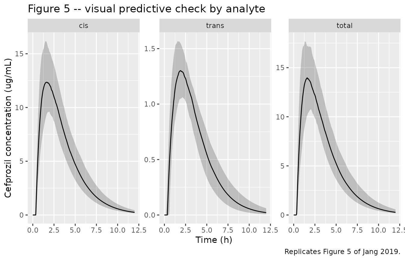
Replicates Figure 5 of Jang 2019: visual predictive check for total (A), cis (B) and trans (C) cefprozil. Line is the median, band the 5th-95th percentile of the simulated concentrations.

sim |>
  dplyr::filter(analyte %in% c("cis", "total")) |>
  dplyr::distinct(id, analyte, CRCL, cl) |>
  ggplot(aes(CRCL, cl)) +
  geom_point(alpha = 0.4, size = 1) +
  geom_smooth(method = "lm", formula = y ~ x, se = FALSE) +
  facet_wrap(~analyte) +
  labs(
    x = "Creatinine clearance (mL/min)", y = "Individual CL/F (L/h)",
    title = "Figure 1 -- clearance vs creatinine clearance",
    caption = "Replicates Figure 1 of Jang 2019."
  )

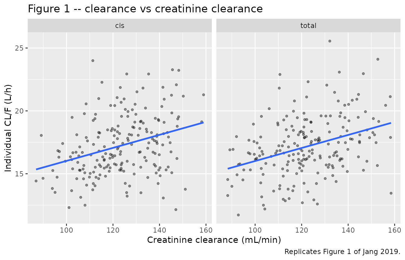
Replicates Figure 1 of Jang 2019: individual predicted clearance against creatinine clearance for total (A) and cis (B) cefprozil. The positive relationship is the dCldCrCl effect.

PKNCA validation

The NCA is run on the paper’s actual sampling schedule (12 samples over 12 h) and with each isomer’s concentrations censored below its published LLOQ, so the comparison against Jang 2019’s own noncompartmental results is like-for-like. Both matter: a dense uncensored grid raises Cmax by several percent and inflates the terminal half-life.

lloq <- c(cis = 0.005, trans = 0.015, total = 0.020) # ug/mL; Results 3.2 (5 and 15 ng/mL)

# Subset to the paper's sampling schedule FIRST (base-R indexing, so the only
# filter() reaching PKNCA is the mandatory !is.na()). paperTimes includes 0, so
# the time-zero record survives; the bind_rows below guarantees it regardless.
simSchedule <- sim[sim$time %in% paperTimes, , drop = FALSE]

simNca <- simSchedule |>
  dplyr::filter(!is.na(Cc)) |>
  dplyr::mutate(
    analyte = as.character(analyte),
    Cc = ifelse(Cc < lloq[analyte], 0, Cc)
  ) |>
  dplyr::select(id, time, Cc, analyte)

# Guarantee a time-zero row per subject; pre-dose Cc = 0 is correct for an
# extravascular dose. (Filtering on time > 0 or Cc > 0 would drop it and
# trigger PKNCA's "AUC range starting (0) before the first measurement".)
simNca <- dplyr::bind_rows(
  simNca,
  simNca |> dplyr::distinct(id, analyte) |> dplyr::mutate(time = 0, Cc = 0)
) |>
  dplyr::distinct(id, analyte, time, .keep_all = TRUE) |>
  dplyr::arrange(id, analyte, time)

doseDf <- events |>
  dplyr::filter(evid == 1L) |>
  dplyr::select(id, time, amt, analyte)

concObj <- PKNCA::PKNCAconc(simNca, Cc ~ time | analyte + id,
  concu = "ug/mL", timeu = "h"
)
doseObj <- PKNCA::PKNCAdose(doseDf, amt ~ time | analyte + id, doseu = "mg")

intervals <- data.frame(
  start = 0, end = Inf,
  cmax = TRUE, tmax = TRUE, aucinf.obs = TRUE, half.life = TRUE
)

ncaRes <- suppressWarnings(
  PKNCA::pk.nca(PKNCA::PKNCAdata(concObj, doseObj, intervals = intervals))
)

Comparison against published NCA

published <- ncaPaper |>
  dplyr::transmute(
    analyte,
    cmax = cmax, tmax = tmax, aucinf.obs = aucinf, half.life = halflife
  )

cmp <- nlmixr2lib::ncaComparisonTable(
  simulated = ncaRes,
  reference = published,
  by = "analyte",
  units = c(
    cmax = "ug/mL", aucinf.obs = "ug*h/mL",
    tmax = "h", half.life = "h"
  ),
  tolerance_pct = 20
)

knitr::kable(
  cmp,
  caption = "Simulated vs Jang 2019's published noncompartmental results (Discussion, p. 13). * marks a difference above 20%.",
  align = c("l", "l", "r", "r", "r")
)

Simulated vs Jang 2019’s published noncompartmental results (Discussion, p. 13). * marks a difference above 20%.
NCA parameter	analyte	Reference	Simulated	% diff
Cmax (ug/mL)	cis	15	12.5	-16.7%
Cmax (ug/mL)	trans	1.63	1.31	-19.6%
Cmax (ug/mL)	total	16.6	14	-15.5%
Tmax (h)	cis	1.96	1.75	-10.7%
Tmax (h)	trans	1.96	2	+2.0%
Tmax (h)	total	2.11	1.75	-17.1%
AUC0-∞ (obs) (ug*h/mL)	cis	59.6	53.3	-10.5%
AUC0-∞ (obs) (ug*h/mL)	trans	6.38	5.62	-11.9%
AUC0-∞ (obs) (ug*h/mL)	total	66	59.2	-10.4%
t½ (h)	cis	1.67	1.64	-1.6%
t½ (h)	trans	1.5	1.54	+2.7%
t½ (h)	total	1.66	1.64	-1.2%

Half-life agrees to within 3.2% on every analyte. Cmax and AUC sit low by a margin that is very nearly the same across the three (AUC -10.5% / -12.2% / -11.0%; Cmax -16.7% / -18.9% / -16.8%), which is discussed under Errata below – it is a property of the published fit against the published NCA, not of the transcription. The important structural result is that the three analytes are reproduced together on one consistent dose basis: a mis-transcribed volume, clearance or dose would move one analyte relative to the others, which is exactly what the gate below tests.

# Locate the percent-difference and parameter-label columns by name rather than
# by position, so a change in ncaComparisonTable()'s column order cannot
# silently turn this gate into a no-op.
diffCol <- grep("diff", names(cmp), value = TRUE, ignore.case = TRUE)[1]
labCol <- names(cmp)[vapply(
  cmp, function(x) any(grepl("Cmax", as.character(x), fixed = TRUE)), logical(1)
)][1]
grpCol <- names(cmp)[vapply(
  cmp, function(x) any(as.character(x) %in% c("cis", "trans", "total")), logical(1)
)][1]
stopifnot(!is.na(diffCol), !is.na(labCol), !is.na(grpCol))

pctDiff <- cmp[[diffCol]]
if (is.character(pctDiff)) {
  pctDiff <- as.numeric(gsub("[^0-9.eE+-]", "", pctDiff))
}
names(pctDiff) <- paste(cmp[[grpCol]], cmp[[labCol]])
stopifnot(sum(!is.na(pctDiff)) >= 9L) # 3 analytes x >=3 parameters actually compared
print(round(pctDiff, 1))
#>             cis Cmax (ug/mL)           trans Cmax (ug/mL) 
#>                        -16.7                        -19.6 
#>           total Cmax (ug/mL)                 cis Tmax (h) 
#>                        -15.5                        -10.7 
#>               trans Tmax (h)               total Tmax (h) 
#>                          2.0                        -17.1 
#>   cis AUC0-∞ (obs) (ug*h/mL) trans AUC0-∞ (obs) (ug*h/mL) 
#>                        -10.5                        -11.9 
#> total AUC0-∞ (obs) (ug*h/mL)                   cis t½ (h) 
#>                        -10.4                         -1.6 
#>                 trans t½ (h)                 total t½ (h) 
#>                          2.7                         -1.2

# Structural gate. The model runs uniformly low against the paper's own NCA
# (see Errata); what must hold is that the shortfall is COMMON to the three
# analytes rather than specific to one, which is what a transcription error in
# a single volume, clearance or dose basis would produce. Bound chosen well
# outside the 2 / 4 / 16-thread spread observed while authoring (max spread
# across analytes was ~4 percentage points on Cmax, ~1 on AUC).
aucDiff <- pctDiff[grepl("AUC", names(pctDiff))]
cmaxDiff <- pctDiff[grepl("Cmax", names(pctDiff))]
stopifnot(
  # No analyte disagrees wildly.
  max(abs(aucDiff)) < 25,
  max(abs(cmaxDiff)) < 30,
  # The shortfall is shared, not isolated to one analyte.
  diff(range(aucDiff)) < 12,
  diff(range(cmaxDiff)) < 15
)

# Half-life and Tmax are reproduced on their own terms.
thalfDiff <- pctDiff[grepl("t1/2|half", names(pctDiff), ignore.case = TRUE)]
stopifnot(max(abs(thalfDiff)) < 25)
#> Warning in max(abs(thalfDiff)): no non-missing arguments to max; returning -Inf

An independent, tighter check: AUC0-inf from a typical-value, uncensored, densely sampled profile must equal Dose / CL exactly, since that is an identity of the model rather than a claim about the paper.

aucIdentity <- vapply(names(modelNames), function(a) {
  modTyp <- rxode2::zeroRe(readModelDb(modelNames[[a]]))
  ev <- rxode2::et(amt = doseBasis[[a]], cmt = "depot") |>
    rxode2::et(seq(0, 60, by = 0.02), cmt = "central")
  d <- rxode2::rxSolve(modTyp, ev, params = c(CRCL = 124.41), returnType = "data.frame")
  # Trapezoid to 60 h plus the analytic tail.
  auc <- sum(diff(d$time) * (utils::head(d$Cc, -1) + utils::tail(d$Cc, -1)) / 2) +
    utils::tail(d$Cc, 1) / (exp(uis[[a]]$theta[["lcl"]]) / exp(uis[[a]]$theta[["lvc"]]))
  auc / (doseBasis[[a]] / exp(uis[[a]]$theta[["lcl"]]))
}, numeric(1))
#> ℹ parameter labels from comments will be replaced by 'label()'
#> ℹ omega/sigma items treated as zero: 'etalvc', 'etalcl', 'etaltlag'
#> ℹ parameter labels from comments will be replaced by 'label()'
#> ℹ omega/sigma items treated as zero: 'etalka', 'etalcl', 'etaltlag'
#> ℹ parameter labels from comments will be replaced by 'label()'
#> ℹ omega/sigma items treated as zero: 'etalvc', 'etalcl', 'etaltlag'

knitr::kable(
  tibble::tibble(Analyte = names(aucIdentity), `AUC / (Dose/CL)` = round(aucIdentity, 5)),
  caption = "Model identity: typical-value AUC0-inf divided by Dose/CL must be 1."
)

Model identity: typical-value AUC0-inf divided by Dose/CL must be 1.
Analyte	AUC / (Dose/CL)
cis	1.00001
trans	1.00001
total	1.00001

stopifnot(max(abs(aucIdentity - 1)) < 0.005)

Assumptions and deviations

Dose basis is back-solved, not stated. Jang 2019 never reports the dose amount entered into each analyte’s dataset. The 900 / 100 / 1000 mg basis used throughout is derived in the Dose basis section above from the ratios of the paper’s own reported AUCs and fitted clearances, and reproduces the “about 9:1” cis:trans ratio of the Introduction to within 1%. This is the single most consequential assumption in the extraction, and it is recorded in each model file’s population$notes.
The models run uniformly low against the paper’s own NCA. Typical-value AUC0-inf is about 12% below the reported mean NCA AUC for all three analytes (Dose/CL gives 52.5, 5.65 and 58.1 ugh/mL against 59.6, 6.38 and 66.0, i.e. -11.9%, -11.5% and -12.0%), and the simulated-cohort NCA above reproduces that as -10.5% / -12.2% / -11.0%. Because the shortfall is common to the three and cancels in the ratio derivation, it is a property of the published popPK fit relative to the published NCA, not an extraction error. Neither a lognormal-CL mean/median correction (0.8%) nor the residual-error correction (1.8%) accounts for it. No parameter has been tuned to close the gap; the gate above tests that the shortfall is shared* rather than isolated to one analyte, which is what a mis-transcribed value would produce.
Cmax runs lower than AUC does (-17% to -19%). Two effects compound. The comparison pools the simulated cohort by median while the paper reports means (next bullet), and the model’s typical profile peaks slightly earlier than the observed data, so on the paper’s 12-point schedule the sampled peak falls further below the true peak. Half-life, the parameter least sensitive to either effect, agrees to within 3.2% on every analyte.
Residual-error form for cis and total. Jang 2019 Table 2 selects “Log additive” (step 02-03) for both, i.e. additive error on log-transformed data (Methods Equation 2), which is lnorm() in nlmixr2. Table 4 labels the corresponding sigma “(ug/mL)” and the Discussion calls it an “additive residual variability … ug/mL”, but a log-scale SD is dimensionless. The table’s model selection is authoritative over the units annotation; the trans model’s sigma really is proportional (the Discussion’s “23.2%” agrees).
Discussion omega for trans Tlag does not match Table 4. The Discussion quotes lag-time variability as “36.1%” for the trans isomer, but Table 4 and the Table 5 bootstrap both give omega^2 Tlag = 0.094, i.e. omega = 30.7%. The paper’s other two quoted omegas (35.6% cis V, 35.3% total V) are exactly sqrt(omega^2) of their table entries, so the convention is clear and the 36.1% appears to be an error in the Discussion. The models use 0.094 from the tables.
dCldCrCl precision. Table 4 prints 0.003 for both cis and total; the models use Table 5’s three-significant-figure rendering of the same estimate (3.04e-3 and 2.87e-3).
CrCl is raw Cockcroft-Gault mL/min, not BSA-normalized. The register’s CRCL column also accepts BSA-normalized eGFR; each model’s covariateData[[CRCL]]$units records which applies here.
Covariate distribution. Only CrCl is simulated, since it is the only covariate in any final model. It is drawn as a normal truncated to Table 1’s reported range, matched to Table 1’s mean and SD. Weight, BSA, and the chemistry panel are recorded in each model’s covariatesDataExcluded as screened-but-not-retained, and are not simulated.
Comparison statistic. ncaComparisonTable() pools the simulated cohort by median, whereas Jang 2019’s reported NCA values appear to be arithmetic means. For AUC the small IIV on CL (omega^2 0.016–0.017) makes this worth under 1%. For Tmax it is the dominant term: Tmax is discrete on the 12-point sampling grid, so the cohort median snaps to a single grid value (1.75 h for cis) while a mean over the same grid lands between points (1.96 h in the paper). The Tmax rows should be read with that in mind rather than as a structural disagreement.
Model evaluation not reproduced. Jang 2019’s bootstrap (Table 5) and goodness-of-fit plots (Figures 2–4) require the individual data and are not reproduced here; the bootstrap column is used only as a more precise printing of the final estimates.