L-arginine (Brussee 2016)
Source:vignettes/articles/Brussee_2016_arginine.Rmd
Brussee_2016_arginine.RmdModel and source
- Citation: Brussee JM, Yeo TW, Lampah DA, Anstey NM, Duffull SB (2016). Pharmacokinetic-Pharmacodynamic Model for the Effect of L-Arginine on Endothelial Function in Patients with Moderately Severe Falciparum Malaria. Antimicrob Agents Chemother 60(1):198-205. doi:10.1128/AAC.01479-15. PK structure adapted from Yeo TW, Lampah DA, Gitawati R, Tjitra E, Kenangalem E, Price RN, Anstey NM, Duffull SB (2008). Pharmacokinetics of L-arginine in adults with moderately severe malaria. Antimicrob Agents Chemother 52(12):4381-4387. doi:10.1128/AAC.00421-08.
- Description: Two-compartment population PKPD model for intravenous L-arginine adjunctive therapy in 73 adults with moderately severe falciparum malaria. Exogenous L-arginine PK is two-compartment IV with allometric scaling on CL and V1 and a multiplicative Papuan-ethnicity effect on CL. Endogenous L-arginine concentration follows a second-order polynomial recovery function indexed from approximately two days before presentation (start of symptoms); lognormal between-subject variability multiplies the typical polynomial. Pharmacodynamic output 1 (exhaled NO, ppb) is linear in the exogenous arginine concentration with a per-subject baseline. Pharmacodynamic output 2 (reactive-hyperemia peripheral-arterial-tonometry index, RH-PAT) is linear in the predicted NO minus its baseline, i.e., linear in the exogenous arginine concentration.
- Article: https://doi.org/10.1128/AAC.01479-15
- Upstream PK structure (Yeo 2008): https://doi.org/10.1128/AAC.00421-08
Brussee 2016 expands the Yeo 2008 two-compartment L-arginine population PK model with two pharmacodynamic biomeasures: exhaled nitric oxide (NO, ppb) measured by breath analyzer, and the reactive-hyperemia peripheral-arterial-tonometry index (RH-PAT, unitless), a validated NO-dependent measure of endothelial function. The model was developed to quantify the time course of L-arginine adjunctive therapy on endothelial function in patients with moderately severe falciparum malaria, and to explore dose / infusion-duration trade-offs for prospective intervention studies in severe malaria.
Population
Brussee 2016 fitted the PKPD model to a pool of two prior studies conducted at the Mitra Masyarakat Hospital in Timika, Papua, Indonesia: an observational cohort of 43 patients receiving saline placebo (Yeo 2008 ref 16, natural-history study) and a non-randomised intervention cohort of 30 patients receiving 3, 6, or 12 g L-arginine as a 30-minute intravenous infusion (Yeo 2008 ref 17, the original L-arginine PK study). Pooled n = 73 adult patients with moderately severe falciparum malaria, age 18-56 years (median 27), weight 42-77 kg (median 57), 66% male, 86% Papuan (the remaining 14% are predominantly mainland-Indonesian transmigrants). All subjects received standard artesunate-based antimalarial therapy. Baseline demographics are tabulated in Brussee 2016 Table 1; the two arms are not significantly different.
The same information is available programmatically via the model’s
population metadata:
rxode2::rxode2(readModelDb("Brussee_2016_arginine"))$meta$population.
Source trace
Each ini() parameter has an in-file trailing comment
pointing to the exact source location in
inst/modeldb/specificDrugs/Brussee_2016_arginine.R. The
table below collects the provenance in one place for review.
| Equation / parameter | Value | Source location |
|---|---|---|
lcl (CL) |
log(30.3) L/h |
Brussee 2016 Table 2, CL |
lvc (V1) |
log(26.6) L |
Brussee 2016 Table 2, V1 |
lvp (V2) |
log(80.1) L |
Brussee 2016 Table 2, V2 |
lq (Q) |
log(22) L/h |
Brussee 2016 Table 2, Q |
e_wt_cl (allometric WT exponent on CL) |
2.47 |
Brussee 2016 Table 2, k1 |
e_wt_vc (allometric WT exponent on V1) |
0.757 |
Brussee 2016 Table 2, k2 |
e_papuan_cl (Papuan multiplicative on CL) |
1.9 |
Brussee 2016 Table 2, f |
lrbase_arg (Arg_0) |
log(6.07) mg/L |
Brussee 2016 Table 2, Arg_0 |
theta_t1 (recovery 1st order) |
0.0365 mg/L/h |
Brussee 2016 Table 2, theta_t1 |
theta_t2 (recovery 2nd order) |
-3.48e-5 mg/L/h^2 |
Brussee 2016 Table 2, theta_t2 |
lrbase_no (BL_NO) |
log(18.2) ppb |
Brussee 2016 Table 3, BL_NO |
lsl_no (SL_NO) |
log(0.0243) ppb/(mg/L) |
Brussee 2016 Table 3, SL_NO |
lrbase_ef (BL_EF) |
log(1.86) |
Brussee 2016 Table 3, BL_EF |
lsl_ef (SL_EF) |
log(0.145) 1/ppb |
Brussee 2016 Table 3, SL_EF |
var(etalcl) (omega^2 CL) |
log(1 + 0.339^2) |
Brussee 2016 Table 2, omega CL 33.9% CV |
var(etalvc) (omega^2 V1) |
log(1 + 0.195^2) |
Brussee 2016 Table 2, omega V1 19.5% CV |
var(etalrbase_arg) (omega^2 Arg_0) |
log(1 + 0.445^2) |
Brussee 2016 Table 2, omega Arg_0 44.5% CV |
var(etalrbase_no) (omega^2 BL_NO) |
log(1 + 0.591^2) |
Brussee 2016 Table 3, omega BL_NO 59.1% CV |
var(etalrbase_ef) (omega^2 BL_EF) |
log(1 + 0.125^2) |
Brussee 2016 Table 3, omega RH-PAT 12.5% CV |
propSd (arginine proportional SD) |
0.286 |
Brussee 2016 Table 2, sigma_prop 28.6% CV |
propSd_NO (NO proportional SD) |
0.355 |
Brussee 2016 Table 3, sigma_prop 35.5% CV |
propSd_EF (RH-PAT proportional SD) |
0.213 |
Brussee 2016 Table 3, sigma_prop 21.3% CV |
2-cmt IV ODE (d/dt(central),
d/dt(peripheral1)) |
n/a | Brussee 2016 / Yeo 2008 Methods (2-cmt structure) |
Endogenous baseline polynomial BL_Arg(t)
|
n/a | Brussee 2016 Eq. 1 |
NO linear model BL_NO + SL_NO * (Arg - BL_Arg)
|
n/a | Brussee 2016 Eq. 2 |
RH-PAT linear model BL_EF + SL_EF * (NO - BL_NO)
|
n/a | Brussee 2016 Eq. 3 |
The endogenous baseline polynomial is indexed to a time origin set at
approximately 2 days prior to presentation (the assumed start of malaria
symptoms). At study time 0 the polynomial is evaluated at 48 h of
symptom duration; in model() this is implemented as
t_sym <- time + 48.
The NO equation reduces to
NO = BL_NO + SL_NO * central / V1 because
E[Arg] - BL_Arg = central / V1 (the exogenous PK
contribution); the endogenous polynomial cancels. Similarly the RH-PAT
equation reduces to
EF = BL_EF + SL_EF * SL_NO * central / V1.
Virtual cohort
Original observed data are not publicly available. The figures below use a virtual cohort built to approximate the published trial demographics: 73 adults at 86% Papuan, weight drawn from a truncated normal around 57 kg, with 4 arms (placebo, 3 g, 6 g, 12 g) sized to match the trial (43, 10, 10, 10).
set.seed(20260609)

make_cohort <- function(n, dose_g, treatment, id_offset = 0L) {
  doses_mg <- dose_g * 1000
  infusion_dur_h <- 0.5
  obs_times <- sort(unique(c(
    0, 0.083, 0.333, 0.5, 0.583, 0.833, 1, 1.5, 2, 3, 4, 5,
    6, 8, 12, 20, 24, 30, 36, 42, 48
  )))
  cohort <- tibble(
    id = id_offset + seq_len(n),
    WT = pmin(pmax(rnorm(n, mean = 57, sd = 8), 42), 77),
    RACE_PAPUAN = as.integer(runif(n) < 0.86),
    treatment = treatment,
    dose_g = dose_g
  )
  if (doses_mg > 0) {
    ev_dose <- cohort |>
      mutate(time = 0, amt = doses_mg, rate = doses_mg / infusion_dur_h,
             cmt = "central", evid = 1L)
  } else {
    ev_dose <- cohort[0, ] |>
      mutate(time = numeric(0), amt = numeric(0), rate = numeric(0),
             cmt = character(0), evid = integer(0))
  }
  ev_obs <- cohort |>
    crossing(time = obs_times, output = c("Cc", "NO", "EF")) |>
    mutate(amt = 0, rate = 0, cmt = output, evid = 0L) |>
    select(-output)
  bind_rows(ev_dose, ev_obs) |>
    arrange(id, time, desc(evid)) |>
    select(id, time, amt, rate, cmt, evid, WT, RACE_PAPUAN, treatment, dose_g)
}

events <- bind_rows(
  make_cohort(43, dose_g =  0, treatment = "Placebo", id_offset =    0L),
  make_cohort(10, dose_g =  3, treatment = "3 g",     id_offset =  100L),
  make_cohort(10, dose_g =  6, treatment = "6 g",     id_offset =  200L),
  make_cohort(10, dose_g = 12, treatment = "12 g",    id_offset =  300L)
)
events$treatment <- factor(events$treatment, levels = c("Placebo", "3 g", "6 g", "12 g"))
stopifnot(!anyDuplicated(unique(events[, c("id", "time", "evid", "cmt")])))
Simulation
Brussee 2016 was developed in NONMEM with FOCE-I; the structural model and IIV / residual variances are reproduced verbatim in the packaged model. Simulation uses rxode2 with the packaged IIV / residual error.
mod <- rxode2::rxode2(readModelDb("Brussee_2016_arginine"))
#> ℹ parameter labels from comments will be replaced by 'label()'
sim <- as.data.frame(
  rxode2::rxSolve(mod, events = events, keep = c("treatment", "dose_g", "WT", "RACE_PAPUAN"))
)
sim$treatment <- factor(sim$treatment, levels = c("Placebo", "3 g", "6 g", "12 g"))
For deterministic typical-value plots (reproducing Brussee 2016 Figure 2 / 3 typical trajectories), zero out the random effects:
mod_typical <- mod |> rxode2::zeroRe()

ev_typ <- function(dose_g, treatment) {
  doses_mg <- dose_g * 1000
  obs_times <- seq(0, 48, by = 0.25)
  cohort <- tibble(
    id = 1L, WT = 57, RACE_PAPUAN = 1L, treatment = treatment, dose_g = dose_g
  )
  if (doses_mg > 0) {
    ev_dose <- cohort |>
      mutate(time = 0, amt = doses_mg, rate = doses_mg / 0.5,
             cmt = "central", evid = 1L)
  } else {
    ev_dose <- cohort[0, ] |>
      mutate(time = numeric(0), amt = numeric(0), rate = numeric(0),
             cmt = character(0), evid = integer(0))
  }
  ev_obs <- cohort |>
    crossing(time = obs_times, output = c("Cc", "NO", "EF")) |>
    mutate(amt = 0, rate = 0, cmt = output, evid = 0L) |>
    select(-output)
  bind_rows(ev_dose, ev_obs) |>
    arrange(id, time, desc(evid)) |>
    select(id, time, amt, rate, cmt, evid, WT, RACE_PAPUAN, treatment, dose_g)
}

sim_typ <- bind_rows(
  as.data.frame(rxode2::rxSolve(mod_typical, events = ev_typ( 0, "Placebo"),
                                keep = c("treatment", "dose_g"))),
  as.data.frame(rxode2::rxSolve(mod_typical, events = ev_typ( 3, "3 g"),
                                keep = c("treatment", "dose_g"))),
  as.data.frame(rxode2::rxSolve(mod_typical, events = ev_typ( 6, "6 g"),
                                keep = c("treatment", "dose_g"))),
  as.data.frame(rxode2::rxSolve(mod_typical, events = ev_typ(12, "12 g"),
                                keep = c("treatment", "dose_g")))
)
#> ℹ omega/sigma items treated as zero: 'etalcl', 'etalvc', 'etalrbase_arg', 'etalrbase_no', 'etalrbase_ef'
#> ℹ omega/sigma items treated as zero: 'etalcl', 'etalvc', 'etalrbase_arg', 'etalrbase_no', 'etalrbase_ef'
#> ℹ omega/sigma items treated as zero: 'etalcl', 'etalvc', 'etalrbase_arg', 'etalrbase_no', 'etalrbase_ef'
#> ℹ omega/sigma items treated as zero: 'etalcl', 'etalvc', 'etalrbase_arg', 'etalrbase_no', 'etalrbase_ef'
sim_typ$treatment <- factor(sim_typ$treatment, levels = c("Placebo", "3 g", "6 g", "12 g"))
Replicate published figures
Figure 2 – arginine, NO, and RH-PAT vs time by dose group
Brussee 2016 Figure 2 shows observed arginine concentrations (panels a-d), exhaled NO (e-h), and RH-PAT index (i-l) over the first 24 hours by dose group. Below are the corresponding typical-value trajectories predicted by the packaged model for a 57 kg Papuan subject. Because the simulation produces all three outputs per time point, we dedupe to one row per (treatment, time) for the deterministic panels.
sim_typ_dedup <- sim_typ |>
  distinct(treatment, dose_g, time, .keep_all = TRUE)
ggplot(sim_typ_dedup, aes(time, Cc, colour = treatment)) +
  geom_line(linewidth = 1) +
  scale_y_log10() +
  coord_cartesian(xlim = c(0, 24)) +
  labs(x = "Time (h)", y = "Arginine concentration (mg/L)",
       title = "Figure 2 (a-d) typical-value reproduction",
       caption = "Replicates the panel structure of Brussee 2016 Figure 2 a-d (arginine).",
       colour = "Dose group")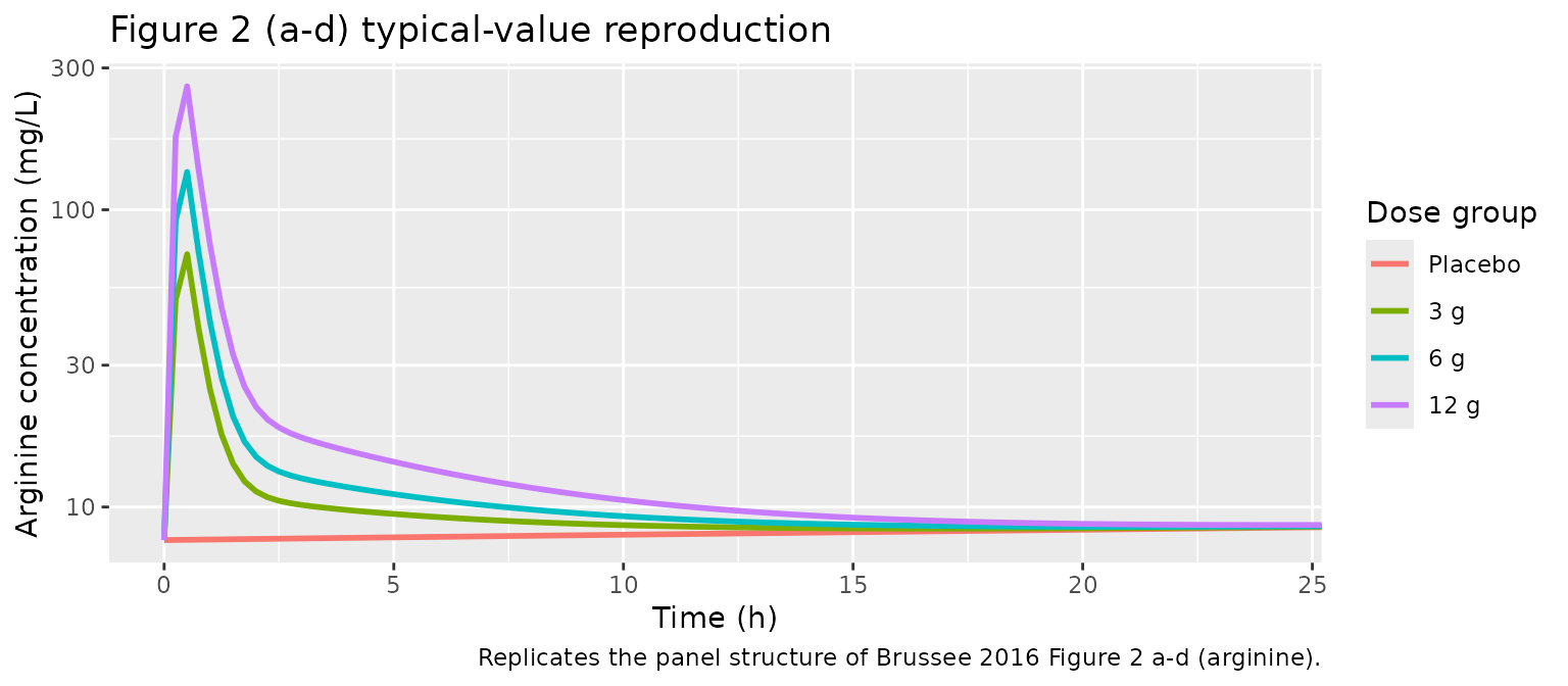
ggplot(sim_typ_dedup, aes(time, NO, colour = treatment)) +
  geom_line(linewidth = 1) +
  coord_cartesian(xlim = c(0, 24)) +
  labs(x = "Time (h)", y = "Exhaled NO (ppb)",
       title = "Figure 2 (e-h) typical-value reproduction",
       caption = "Replicates the panel structure of Brussee 2016 Figure 2 e-h (NO).",
       colour = "Dose group")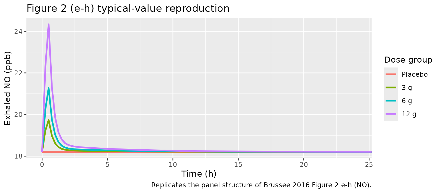
ggplot(sim_typ_dedup, aes(time, EF, colour = treatment)) +
  geom_line(linewidth = 1) +
  coord_cartesian(xlim = c(0, 24)) +
  labs(x = "Time (h)", y = "RH-PAT index (unitless)",
       title = "Figure 2 (i-l) typical-value reproduction",
       caption = "Replicates the panel structure of Brussee 2016 Figure 2 i-l (RH-PAT).",
       colour = "Dose group")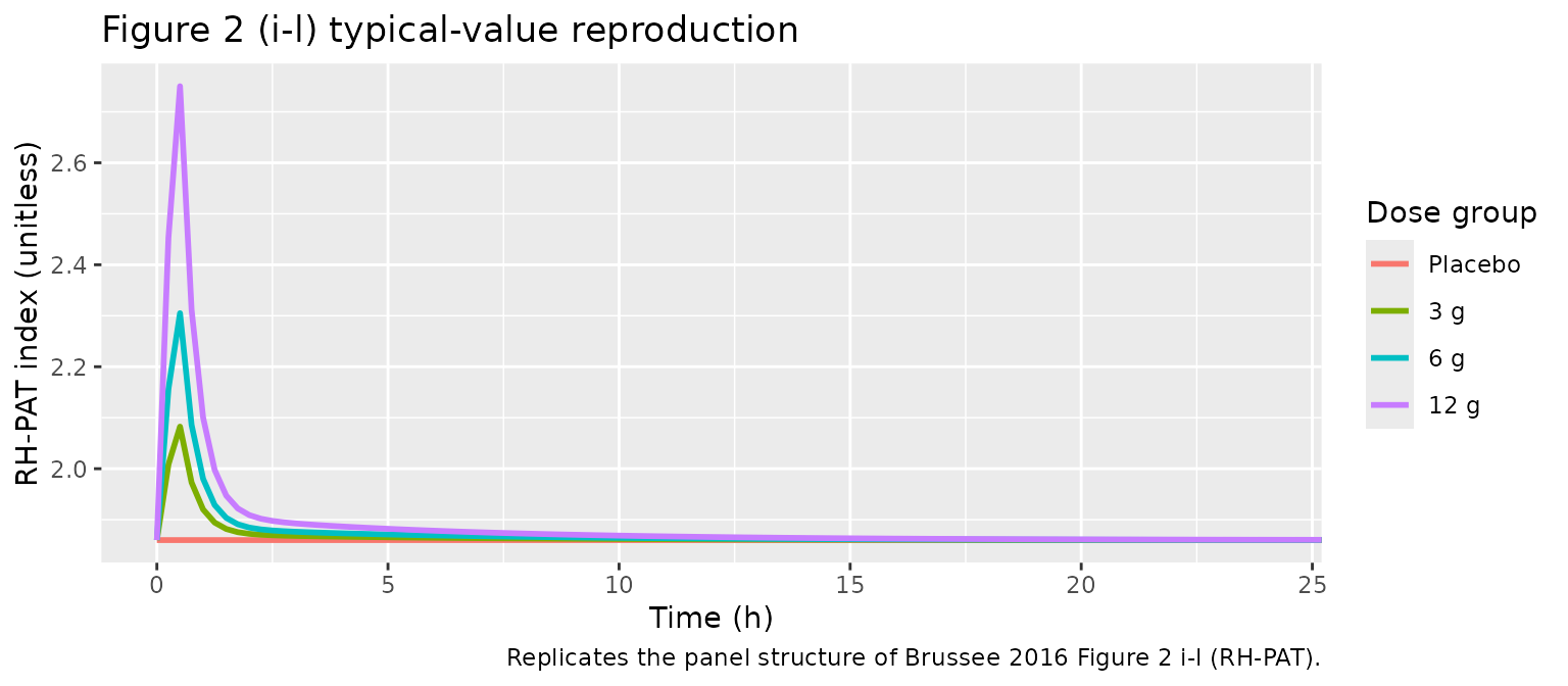
Figure 3 – VPC for arginine, NO, and RH-PAT
Brussee 2016 Figure 3 shows VPCs of the three measurements for the pooled cohort. The cohort below pools all 73 simulated subjects (43 placebo + 30 active across three dose groups) so the VPC describes the full pooled study population, matching the analysis dataset. Each simulated row is deduped to one observation per (id, time) so that each subject contributes a single trajectory per output.
sim_dedup <- sim |>
  distinct(id, time, .keep_all = TRUE)

vpc_long <- sim_dedup |>
  select(id, time, treatment, Cc, NO, EF) |>
  pivot_longer(c(Cc, NO, EF), names_to = "output", values_to = "value")

vpc_summary <- vpc_long |>
  group_by(output, time) |>
  summarise(
    Q10 = quantile(value, 0.10, na.rm = TRUE),
    Q50 = quantile(value, 0.50, na.rm = TRUE),
    Q90 = quantile(value, 0.90, na.rm = TRUE),
    .groups = "drop"
  ) |>
  mutate(panel = factor(output,
                        levels = c("Cc", "NO", "EF"),
                        labels = c("Arginine (mg/L)", "NO (ppb)", "RH-PAT")))

ggplot(vpc_summary, aes(time, Q50)) +
  geom_ribbon(aes(ymin = Q10, ymax = Q90), alpha = 0.25) +
  geom_line(linewidth = 0.8) +
  facet_wrap(~panel, scales = "free_y") +
  labs(x = "Time (h)", y = "Concentration / index",
       title = "Figure 3 reproduction -- VPC for pooled cohort",
       caption = "Replicates the panel structure of Brussee 2016 Figure 3 (VPC arginine | NO | RH-PAT).")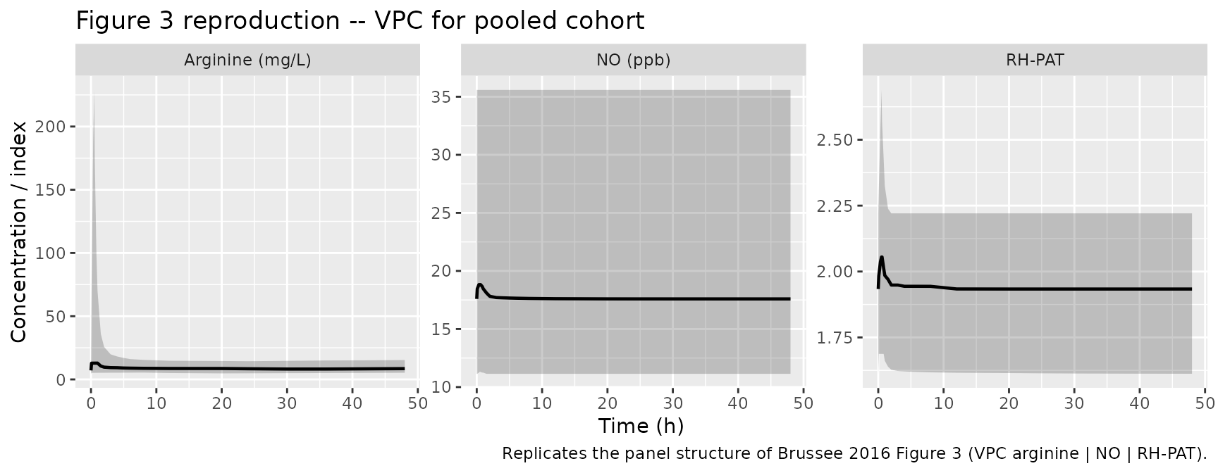
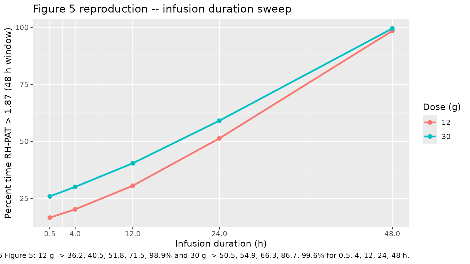
Figures 4 and 5 – dose / infusion-duration response
Brussee 2016 Figure 4 shows the percentage of time within the RH-PAT therapeutic range (above 1.87) for 3, 6, 12, and 30 g half-hour infusions, and Figure 5 shows the same metric for 12 g and 30 g administered as 0.5, 4, 12, 24, and 48 h infusions. The chunk below reproduces the percent-time-in-therapeutic-range curve for half-hour infusions of 3, 6, 12, and 30 g and the 12 g / 30 g infusion-duration sweep.
make_typ_events <- function(dose_g, dur_h) {
  doses_mg <- dose_g * 1000
  obs_times <- seq(0, 48, by = 0.25)
  cohort <- tibble(id = 1L, WT = 60, RACE_PAPUAN = 1L)
  if (doses_mg > 0) {
    ev_dose <- cohort |>
      mutate(time = 0, amt = doses_mg, rate = doses_mg / dur_h,
             cmt = "central", evid = 1L)
  } else {
    ev_dose <- cohort[0, ] |>
      mutate(time = numeric(0), amt = numeric(0), rate = numeric(0),
             cmt = character(0), evid = integer(0))
  }
  ev_obs <- cohort |>
    crossing(time = obs_times, output = c("Cc", "NO", "EF")) |>
    mutate(amt = 0, rate = 0, cmt = output, evid = 0L) |>
    select(-output)
  bind_rows(ev_dose, ev_obs) |>
    arrange(id, time, desc(evid))
}

pct_above <- function(dose_g, dur_h, threshold = 1.87) {
  ev <- make_typ_events(dose_g, dur_h)
  sim <- as.data.frame(rxode2::rxSolve(mod_typical, events = ev))
  sim_ef <- sim |> filter(!is.na(EF))
  mean(sim_ef$EF > threshold) * 100
}

fig4 <- tibble(
  dose_g = c(3, 6, 12, 30),
  dur_h  = 0.5
) |>
  rowwise() |>
  mutate(pct_time_above = pct_above(dose_g, dur_h)) |>
  ungroup()
#> ℹ omega/sigma items treated as zero: 'etalcl', 'etalvc', 'etalrbase_arg', 'etalrbase_no', 'etalrbase_ef'
#> ℹ omega/sigma items treated as zero: 'etalcl', 'etalvc', 'etalrbase_arg', 'etalrbase_no', 'etalrbase_ef'
#> ℹ omega/sigma items treated as zero: 'etalcl', 'etalvc', 'etalrbase_arg', 'etalrbase_no', 'etalrbase_ef'
#> ℹ omega/sigma items treated as zero: 'etalcl', 'etalvc', 'etalrbase_arg', 'etalrbase_no', 'etalrbase_ef'

ggplot(fig4, aes(factor(dose_g), pct_time_above)) +
  geom_col(fill = "steelblue4") +
  geom_text(aes(label = sprintf("%.1f%%", pct_time_above)), vjust = -0.4) +
  labs(x = "L-arginine dose (g, 0.5 h infusion)",
       y = "Percent time RH-PAT > 1.87 (48 h window)",
       title = "Figure 4 reproduction -- percent time above therapeutic threshold",
       caption = paste0(
         "Brussee 2016 Figure 4 reports 14.8%, 25.6%, 36.2%, 50.5% for 3, 6, 12, 30 g."
       ))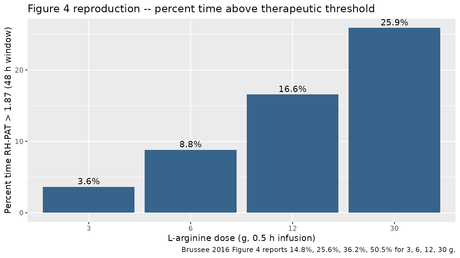
fig5 <- tibble(
  dose_g = rep(c(12, 30), each = 5),
  dur_h  = rep(c(0.5, 4, 12, 24, 48), 2)
) |>
  rowwise() |>
  mutate(pct_time_above = pct_above(dose_g, dur_h)) |>
  ungroup()
#> ℹ omega/sigma items treated as zero: 'etalcl', 'etalvc', 'etalrbase_arg', 'etalrbase_no', 'etalrbase_ef'
#> ℹ omega/sigma items treated as zero: 'etalcl', 'etalvc', 'etalrbase_arg', 'etalrbase_no', 'etalrbase_ef'
#> ℹ omega/sigma items treated as zero: 'etalcl', 'etalvc', 'etalrbase_arg', 'etalrbase_no', 'etalrbase_ef'
#> ℹ omega/sigma items treated as zero: 'etalcl', 'etalvc', 'etalrbase_arg', 'etalrbase_no', 'etalrbase_ef'
#> ℹ omega/sigma items treated as zero: 'etalcl', 'etalvc', 'etalrbase_arg', 'etalrbase_no', 'etalrbase_ef'
#> ℹ omega/sigma items treated as zero: 'etalcl', 'etalvc', 'etalrbase_arg', 'etalrbase_no', 'etalrbase_ef'
#> ℹ omega/sigma items treated as zero: 'etalcl', 'etalvc', 'etalrbase_arg', 'etalrbase_no', 'etalrbase_ef'
#> ℹ omega/sigma items treated as zero: 'etalcl', 'etalvc', 'etalrbase_arg', 'etalrbase_no', 'etalrbase_ef'
#> ℹ omega/sigma items treated as zero: 'etalcl', 'etalvc', 'etalrbase_arg', 'etalrbase_no', 'etalrbase_ef'
#> ℹ omega/sigma items treated as zero: 'etalcl', 'etalvc', 'etalrbase_arg', 'etalrbase_no', 'etalrbase_ef'

ggplot(fig5, aes(dur_h, pct_time_above, colour = factor(dose_g))) +
  geom_line(linewidth = 1) +
  geom_point(size = 2) +
  scale_x_continuous(breaks = c(0.5, 4, 12, 24, 48)) +
  labs(x = "Infusion duration (h)",
       y = "Percent time RH-PAT > 1.87 (48 h window)",
       title = "Figure 5 reproduction -- infusion duration sweep",
       colour = "Dose (g)",
       caption = paste0(
         "Brussee 2016 Figure 5: 12 g -> 36.2, 40.5, 51.8, 71.5, 98.9% and ",
         "30 g -> 50.5, 54.9, 66.3, 86.7, 99.6% for 0.5, 4, 12, 24, 48 h."
       ))
PKNCA validation
NCA is not reported in Brussee 2016 (the paper publishes only
structural parameter estimates and VPC figures). The block below
computes a per-dose NCA summary on the simulated exogenous
L-arginine concentration (central / vc, i.e. the
model-predicted arginine concentration minus the endogenous polynomial
baseline) for the three active dose groups.
sim_exo <- sim |>
  distinct(id, time, .keep_all = TRUE) |>
  filter(treatment != "Placebo") |>
  mutate(Cc_exo = central / vc) |>
  select(id, time, Cc_exo, treatment)

dose_df <- events |>
  filter(evid == 1, treatment != "Placebo") |>
  select(id, time, amt, treatment)

conc_obj <- PKNCA::PKNCAconc(sim_exo, Cc_exo ~ time | treatment + id,
                             concu = "mg/L", timeu = "hour")
dose_obj <- PKNCA::PKNCAdose(dose_df, amt ~ time | treatment + id,
                             doseu = "mg")

intervals <- data.frame(
  start       = 0,
  end         = Inf,
  cmax        = TRUE,
  tmax        = TRUE,
  aucinf.obs  = TRUE,
  half.life   = TRUE
)

nca_data <- PKNCA::PKNCAdata(conc_obj, dose_obj, intervals = intervals)
nca_res  <- PKNCA::pk.nca(nca_data)
nca_summary <- summary(nca_res)
knitr::kable(nca_summary,
caption = "Simulated NCA for exogenous L-arginine by dose group.")| Interval Start | Interval End | treatment | N | Cmax (mg/L) | Tmax (hour) | Half-life (hour) | AUCinf,obs (hour*mg/L) |
|---|---|---|---|---|---|---|---|
| 0 | Inf | 3 g | 10 | 66.5 [25.1] | 0.500 [0.500, 0.500] | 4.49 [1.76] | 75.1 [70.5] |
| 0 | Inf | 6 g | 10 | 119 [21.6] | 0.500 [0.500, 0.500] | 4.13 [0.923] | 136 [49.1] |
| 0 | Inf | 12 g | 10 | 264 [27.5] | 0.500 [0.500, 0.500] | 4.20 [1.06] | 281 [58.7] |
Comparison against published NCA
Brussee 2016 does not tabulate NCA parameters. The Yeo 2008 upstream
PK paper (AAC 52(12):4381) reports L-arginine clearance of ~30 L/h in
the moderately severe malaria cohort, which corresponds to a terminal
half-life of approximately
log(2) * (V1 + V2) / CL = log(2) * (26.6 + 80.1) / 30.3 = 2.44 h.
The PKNCA half-life above should land near this value for a
typical-weight non-Papuan subject; Papuan subjects have approximately
1.9-fold higher CL and a correspondingly shorter half-life.
Assumptions and deviations
- The endogenous baseline polynomial in
BL_Arg(t)is indexed to the start of malaria symptoms, taken in the paper as approximately 2 days before presentation. The packaged model implements this by evaluating the polynomial att_sym = time + 48(hours). Subjects who present with a substantially different symptom-duration history would need the 48 h offset adjusted; the offset is hard-coded inmodel()and is not aini()parameter. - The lognormal random effect on the endogenous baseline
(
etalrbase_arg,omega_Arg_0 = 44.5% CV) multiplies the entire typical polynomial per the paper’s Eq. 1: `BL_Arg(t)_i = (Arg_0 + theta_t1 * t + theta_t2- t^2) * exp(eta_1_i)`. The packaged model reproduces this exactly.
- Brussee 2016 fits a combined (additive + proportional)
residual-error model for each of the three outputs with the additive
component fixed at approximately zero (
sigma_add ~= 0 FIX, Tables 2 and 3). The packaged model encodes this as proportional-only, since the additive component carries no estimated information in the source. - Race / ethnicity is encoded via a single binary
RACE_PAPUANindicator. The Brussee 2016 cohort was enrolled exclusively at one Papuan site, so the non-Papuan reference category is predominantly mainland-Indonesian transmigrants of Austronesian (Asian) descent. Users applying this model to other populations should reconsider the reference category accordingly. - The Brussee 2016 PK structure inherits from Yeo 2008 (AAC
52(12):4381). Both papers use the same Papuan-vs-non-Papuan
multiplicative-on-CL covariate; the WT allometric exponents
k1andk2were re-estimated in Brussee 2016 with the expanded PD dataset (one row in Table 2). When using this model, refer to Yeo 2008 for the PK-only validation precedent. - Time-varying body weight is not described in Brussee 2016 (Table 1
reports a single weight). The packaged model treats
WTas a baseline (time-fixed) covariate.