Malabsorption blood test: pentadecanoic and triheptadecanoic acid (Mascarenhas 2015)
Source:vignettes/articles/Mascarenhas_2015_pentadecanoic_triheptadecanoic.Rmd
Mascarenhas_2015_pentadecanoic_triheptadecanoic.RmdModel and source
mod <- rxode2::rxode(readModelDb("Mascarenhas_2015_pentadecanoic_triheptadecanoic"))
#> ℹ parameter labels from comments will be replaced by 'label()'
#> Warning: some etas defaulted to non-mu referenced, possible parsing error: etaiov_mtt_1, etaiov_mtt_2, etaiov_mtt_3, etaiov_mtt_4, etaiov_fdepot_1, etaiov_fdepot_2, etaiov_fdepot_3, etaiov_fdepot_4, etaiov_mtt_hepta_1, etaiov_mtt_hepta_2, etaiov_mtt_hepta_3, etaiov_mtt_hepta_4, etaiov_fdepot_hepta_1, etaiov_fdepot_hepta_2, etaiov_fdepot_hepta_3, etaiov_fdepot_hepta_4
#> as a work-around try putting the mu-referenced expression on a simple line
mod_typical <- rxode2::zeroRe(mod)
#> Warning: some etas defaulted to non-mu referenced, possible parsing error: etaiov_mtt_1, etaiov_mtt_2, etaiov_mtt_3, etaiov_mtt_4, etaiov_fdepot_1, etaiov_fdepot_2, etaiov_fdepot_3, etaiov_fdepot_4, etaiov_mtt_hepta_1, etaiov_mtt_hepta_2, etaiov_mtt_hepta_3, etaiov_mtt_hepta_4, etaiov_fdepot_hepta_1, etaiov_fdepot_hepta_2, etaiov_fdepot_hepta_3, etaiov_fdepot_hepta_4
#> as a work-around try putting the mu-referenced expression on a simple line- Citation: Mascarenhas MR, Mondick J, Barrett JS, Wilson M, Stallings VA, Schall JI. Malabsorption Blood Test: Assessing Fat Absorption in Patients With Cystic Fibrosis and Pancreatic Insufficiency. J Clin Pharmacol. 2015;55(8):854-865. doi:10.1002/jcph.484
- Description: Simultaneous two-analyte population PK model for the malabsorption blood test (MBT) in healthy subjects and subjects with cystic fibrosis and pancreatic insufficiency (Mascarenhas 2015). The MBT co-administers pentadecanoic acid (PA, C15:0), a free fatty acid absorbed without pancreatic lipase, and triheptadecanoic acid (THA), a triglyceride that must be hydrolysed by lipase to release heptadecanoic acid (HA, C17:0) before absorption; the postdose difference between the two analytes measures pancreatic-based fat absorption. Each analyte has its own 1-compartment disposition, its own Savic 2007 analytical transit-compartment absorption chain, and its own estimated fasting baseline concentration added to the model prediction. Allometric body-weight scaling on CL/F and V/F at a 70 kg reference (exponents fixed at 0.75 and 1). Healthy subjects are the bioavailability reference (F = 1); subjects with cystic fibrosis take a relative bioavailability that depends on whether pancreatic enzymes were administered and, for heptadecanoic acid only, on the timing of the enzyme dose relative to the meal. The heptadecanoic-acid random effects are modelled as scaled multiples of the pentadecanoic-acid random effects (correlations 0.974-0.999), and between-occasion variability is carried on mean transit time and on bioavailability for both analytes.
- Article: https://doi.org/10.1002/jcph.484
The malabsorption blood test (MBT) is a diagnostic test meal, not a therapy. It co-administers two odd-chain fatty acids that differ in exactly one respect: pentadecanoic acid (PA, C15:0) is a free fatty acid that is absorbed without pancreatic lipase, while heptadecanoic acid (HA, C17:0) must first be liberated by lipase hydrolysis of the co-administered triglyceride triheptadecanoic acid (THA). The postdose difference between the two plasma profiles is therefore a direct read-out of pancreatic-based fat absorption, and it is the contrast between the analytes – not either concentration alone – that carries the clinical information.
Mascarenhas 2015 fits both analytes simultaneously in a single NONMEM
VII model. Pentadecanoic acid is the unsuffixed parent throughout this
model file; heptadecanoic acid carries the registered
_hepta suffix.
Population
Sixty subjects contributed to the pooled analysis: 33 with cystic fibrosis and pancreatic insufficiency (fecal elastase 1 < 200 ug/g stool, FEV1 >= 40% predicted) and 27 healthy comparison subjects. The CF cohort was substantially younger and lighter than the healthy cohort (median 15.6 years / 50.5 kg versus 28.2 years / 71.6 kg), which matters for the allometric scaling: the CF-versus-healthy bioavailability contrast is estimated after body size has been accounted for at a 70 kg reference.
knitr::kable(
  tibble::tibble(
    Field = names(mod$meta$population),
    Value = vapply(mod$meta$population, function(x) paste(format(x), collapse = "; "), character(1))
  ),
  caption = "Population metadata (Mascarenhas 2015 Table 1 and Methods)."
)| Field | Value |
|---|---|
| species | human |
| n_subjects | 60 |
| n_studies | 5 |
| age_range | 9.9-49.9 years (CF 9.9-24.2; healthy 19.0-49.9) |
| age_median | CF 15.6 years; healthy 28.2 years |
| weight_range | 30.7-101.6 kg (CF 30.7-74.5; healthy 60.0-101.6) |
| weight_median | CF 50.5 kg; healthy 71.6 kg |
| sex_female_pct | 50 |
| disease_state | 33 subjects with cystic fibrosis and pancreatic insufficiency (fecal elastase 1 < 200 ug/g stool, FEV1 >= 40% predicted, no fibrosing colonopathy or significant bowel resection) and 27 healthy comparison subjects (BMI 21-30 kg/m2, no chronic illness affecting nutrient absorption). |
| dose_range | Single oral MBT test meal (8 oz, 550 kcal, 32 g fat) containing 2.5 or 5.0 g pentadecanoic acid and 5.0, 5.5 or 8.0 g triheptadecanoic acid. Healthy Orlistat Protocol 2.5 g PA + 8.0 g THA; healthy Timing Protocol 5.0 g PA + 5.5 g THA; CF No Enzymes Protocol 2.5 g PA + 5.0 g (n=3) or 8.0 g (n=3) THA; CF Timing and Reproducibility Protocols 5.0 g PA + 5.5 g THA. 5.0 g PA + 5.5 g THA was selected as the final MBT. |
| regions | United States (Children’s Hospital of Philadelphia and Pennsylvania Presbyterian Medical Center) |
| co_medication | CF subjects received Creon 20 pancrelipase, 4-7 capsules (80 000-140 000 lipase units): 52% took 80 000 units, 15% 100 000, 21% 120 000, 12% 140 000. Enzymes were taken with the MBT and again with the 6-hour lunch meal, except on the no-enzyme occasion and on the timing-arm occasions where the dose was displaced by -30, +30 or +60 minutes. |
| studies | Pooled analysis across 5 protocols: CF No Enzymes (n=6, 2 occasions), CF Timing of Enzymes (n=16, 3-4 occasions), CF Reproducibility (n=11, 3 occasions), healthy Orlistat (n=15, pre-Orlistat MBT only), healthy Timing of Enzymes comparison group (n=12). |
| notes | Baseline demographics from Mascarenhas 2015 Table 1. Plasma sampled hourly over 8 hours starting with a premeal baseline sample, after a 12-hour overnight fast; subjects abstained from alcohol and dairy for 24 hours beforehand. Estimation in NONMEM VII level 2.0 with FOCE-INT. Parameter precision from a 500-replicate nonparametric bootstrap stratified by subject status and enzyme administration method. sex_female_pct is the pooled figure across both cohorts (CF 45%, healthy 56%). |
The MBT was repeated on up to four separate occasions at least five days apart, which is what makes the between-occasion variability terms estimable.
Structural model
Each analyte has its own one-compartment disposition fed by its own Savic 2007 analytical transit-compartment chain, plus its own estimated fasting baseline concentration:
d/dt(depot)         = transit(nn, mtt, fdepot) - ka * depot
d/dt(central)       = ka * depot - cl/vc * central
Cc                  = central/vc + rbase

d/dt(depot_hepta)   = transit(nn_hepta, mtt_hepta, fdepot_hepta) - ka_hepta * depot_hepta
d/dt(central_hepta) = ka_hepta * depot_hepta - cl_hepta/vc_hepta * central_hepta
Cc_hepta            = central_hepta/vc_hepta + rbase_hepta
Relative bioavailability is the covariate-driven part of the model and is where the whole diagnostic lives. Healthy subjects are the reference (F = 1 for both analytes). For subjects with CF:
| Analyte | No enzymes | Enzymes with the MBT | Enzyme timing |
|---|---|---|---|
| Pentadecanoic acid | 1.07 | 0.877 | no effect |
| Heptadecanoic acid | 0.0292 | 0.606 | x 0.911 (-30 min), x 0.829 (+30 min), x 0.78 (+60 min) |
Both analyte’s random effects are shared: Cc_hepta’s
CL/F, V/F and baseline etas are the corresponding pentadecanoic-acid
etas multiplied by an estimated scale factor, because the source fit
found correlations of 0.974, 0.987 and 0.999 between them.
Dose units
Concentrations are micromol/L and V/F is in litres, so doses must be supplied in micromoles. Each THA molecule carries three heptadecanoic acids, so the molar HA dose is three times the molar THA dose:
MW_PA  <- 242.40  # pentadecanoic acid, C15H30O2
MW_THA <- 849.42  # triheptadecanoic acid (glycerol tri-C17:0)

pa_umol <- function(g_pa)   g_pa  / MW_PA  * 1e6
ha_umol <- function(g_tha)  g_tha / MW_THA * 3 * 1e6

# The final selected MBT (Mascarenhas 2015 Discussion: "we chose 5.0 g of PA
# and 5.5 g of THA") is very nearly equimolar in the two analytes, which is
# the design rationale and is only true under the 3:1 THA -> HA conversion.
c(PA_umol = pa_umol(5.0), HA_umol = ha_umol(5.5))
#>  PA_umol  HA_umol
#> 20627.06 19425.02
Source trace
Every value in ini() comes from Mascarenhas 2015 Table 2
unless noted.
| Model quantity | Source location | Value |
|---|---|---|
lcl, lvc
|
Table 2, PA Estimate | 9.66 L/h, 24.5 L |
lrbase |
Table 2, PA C0 | 24.9 umol/L |
lmtt, lka, lnn
|
Table 2, PA | 0.817 h, 0.266 1/h, 6.96 |
lcl_hepta, lvc_hepta
|
Table 2, HA Estimate | 16.3 L/h, 14.3 L |
lrbase_hepta |
Table 2, HA C0 | 27.4 umol/L |
lmtt_hepta, lka_hepta,
lnn_hepta
|
Table 2, HA | 3.52 h, 0.307 1/h, 7.08 |
e_wt_cl, e_wt_vc
|
Results, allometric model, 70 kg reference | 0.75, 1.0 (fixed) |
e_cf_fdepot, e_cf_enz_fdepot
|
Table 2, PA F_CF / F_CF,ENZ | 1.07, 0.877 |
e_cf_fdepot_hepta,
e_cf_enz_fdepot_hepta
|
Table 2, HA F_CF / F_CF,ENZ | 0.0292, 0.606 |
e_pre30/post30/post60_fdepot_hepta |
Table 2, HA F_T1 / F_T2 / F_T3 | 0.911, 0.829, 0.78 |
cl_hepta_eta_scale, vc_hepta_eta_scale,
rbase_hepta_eta_scale
|
Table 2, theta20 / 21 / 22 | 0.994, 1.3, 0.998 |
| 3x3 IIV block | Table 2, Interindividual variance rows | 0.315, 0.162, 0.341, -0.0894, -0.151, 0.143 |
| IOV on MTT / F, both analytes | Table 2, Intraindividual variance rows | 0.205 / 0.0925 (PA), 0.102 / 0.136 (HA) |
propSd, propSd_hepta
|
Table 2, Residual variance | sqrt(0.0984), sqrt(0.0774) |
| Structural equations | Page 858 final-model equation block | – |
| Dose amounts | Methods, MBT Preparation; Table 1 | – |
Reading Table 2 through a Symbol-font PDF
Two transcription hazards in this article are worth recording, because both are silent and both would corrupt the model.
The text layer of this PDF is lossy in two specific ways, and both
are visible on the Table 2 page itself. It mis-decodes the Symbol-font
micro sign as a Latin “m”, and it silently drops minus
signs: the Ka unit h^-1 extracts as
h1, and the F_T1 row description
“bioavailability effect – enzymes at -0.5 h” extracts as “enzymes at 0.5
h”, which would make it indistinguishable from the F_T2
row. Rendering the page as an image resolves both.
The concentration unit is micromol/L, not mmol/L.
The units column renders as umol/L; the extracted
mmol/L is the mis-decoded micro sign. Two independent facts
agree: the assay quality-control concentrations in Methods (Sample
Analysis) are given in mg/dL, and the highest PA control of 6.70 mg/dL
is 6.70 x 10 / 242.40 = 276 umol/L, which is the scale of the plotted
profiles; and a mmol/L reading would place the fasting baseline of a
plasma fatty acid three orders of magnitude too high.
Two covariances in the interindividual block are
negative. The rendered table prints them as
-0.0894 and -0.151, with relative standard
errors -51.7% and -53.8% and confidence
intervals (-0.162, -0.0259) and
(-0.231, -0.0899). The text layer alone is enough to catch
this even without rendering: those two intervals extract as
(0.162, 0.0259) and (0.231, 0.0899), which are
descending and therefore impossible for a 2.5th-97.5th
bootstrap quantile pair. Both signs are mechanistically sensible – a
subject with higher clearance has a lower baseline concentration – and
the resulting matrix is positive definite:
om <- matrix(c( 0.315,  0.162, -0.0894,
                0.162,  0.341, -0.151,
               -0.0894, -0.151, 0.143), nrow = 3, byrow = TRUE)
c(leading_minors = c(om[1, 1], det(om[1:2, 1:2]), det(om)),
  min_eigenvalue = min(eigen(om)$values))
#> leading_minors1 leading_minors2 leading_minors3  min_eigenvalue
#>     0.315000000     0.081171000     0.006073549     0.061422192
stopifnot(all(eigen(om)$values > 0))
A further consistency check: every variance in Table 2 is reported alongside a percentage, and each percentage is the square root of the variance, confirming that the table reports variances on the log scale and that the printed BSV / BOV columns are the corresponding standard deviations.
vars <- c(CL = 0.315, V = 0.341, C0 = 0.143, MTT_PA = 0.205, MTT_HA = 0.102,
          F_PA = 0.0925, F_HA = 0.136, resid_PA = 0.0984, resid_HA = 0.0774)
printed <- c(56.1, 58.4, 37.8, 45.3, 31.9, 30.4, 36.9, 31.4, 27.8)
chk <- tibble::tibble(term = names(vars), variance = vars,
                      sqrt_pct = round(100 * sqrt(vars), 1), printed_pct = printed)
knitr::kable(chk, caption = "Every Table 2 variance matches its printed percentage as a standard deviation.")| term | variance | sqrt_pct | printed_pct |
|---|---|---|---|
| CL | 0.3150 | 56.1 | 56.1 |
| V | 0.3410 | 58.4 | 58.4 |
| C0 | 0.1430 | 37.8 | 37.8 |
| MTT_PA | 0.2050 | 45.3 | 45.3 |
| MTT_HA | 0.1020 | 31.9 | 31.9 |
| F_PA | 0.0925 | 30.4 | 30.4 |
| F_HA | 0.1360 | 36.9 | 36.9 |
| resid_PA | 0.0984 | 31.4 | 31.4 |
| resid_HA | 0.0774 | 27.8 | 27.8 |
Virtual cohort
# rxode2 returns each declared endpoint on its own observation row. This model
# declares two endpoints (Cc and Cc_hepta), so observation rows are addressed
# by ODE state plus dvid -- the form the naming conventions mandate. All three
# spellings (dvid alone, cmt = observable, cmt = ODE state + dvid) were tested
# against this model and all three solve; the ODE-state form is used here.
# predDf maps dvid 1 -> Cc (cmt 5) and dvid 2 -> Cc_hepta (cmt 6).
knitr::kable(mod$predDf[, c("cond", "var", "cmt", "dvid")],
caption = "Endpoint map for the two declared analytes.")| cond | var | cmt | dvid |
|---|---|---|---|
| Cc | Cc | 5 | 1 |
| Cc_hepta | Cc_hepta | 6 | 2 |
OBS_TIMES <- seq(0, 8, by = 0.25)

# Build a plain data frame: covariate columns assigned onto an rxEt object are
# silently dropped by rxode2.
mbt_events <- function(id, wt, g_pa, g_tha, dis_cf, enz,
                       pre30 = 0, post30 = 0, post60 = 0, occ = 1,
                       times = OBS_TIMES) {
  dose <- data.frame(
    time = 0,
    amt  = c(pa_umol(g_pa), ha_umol(g_tha)),
    cmt  = c("depot", "depot_hepta"),
    evid = 1L, dvid = NA_integer_
  )
  obs <- data.frame(
    time = rep(times, 2L),
    amt  = NA_real_,
    cmt  = rep(c("central", "central_hepta"), each = length(times)),
    evid = 0L,
    dvid = rep(c(1L, 2L), each = length(times))
  )
  out <- dplyr::bind_rows(dose, obs)
  out$id <- id
  out$WT <- wt
  out$DIS_CF <- dis_cf
  out$CONMED_PANCRELIPASE <- enz
  out$CONMED_PANCRELIPASE_PRE30 <- pre30
  out$CONMED_PANCRELIPASE_POST30 <- post30
  out$CONMED_PANCRELIPASE_POST60 <- post60
  out$OCC <- occ
  out[order(out$time, -out$evid), ]
}

# rxSolve labels each output row by the endpoint's predDf$cmt value (5 = Cc,
# 6 = Cc_hepta); there is no dvid column in the output.
label_endpoint <- function(d) {
  d$analyte <- ifelse(d$CMT == 5, "Pentadecanoic acid", "Heptadecanoic acid")
  d
}

# rxSolve() on an rxUi (which is what readModelDb() yields) is quadratic in the
# number of subjects passed in a SINGLE call -- 900 subjects in one call takes
# ~400 s on rxode2 5.1.7 where the same event grid split into 200-subject
# batches takes a few seconds each. Solving one arm at a time keeps the render
# inside its time budget without shrinking the cohort. Subject IDs are disjoint
# across arms, so the only difference from a single call is which eta draw lands
# on which subject.
#
# Reseeding before each arm also gives the cohort COMMON RANDOM NUMBERS: subject
# i draws the same random effects in every arm, so an inter-arm contrast becomes
# a *paired* comparison in which those random effects cancel. That is what makes
# the enzyme-timing checks below exact rather than merely on-average -- see
# "Paired enzyme-timing contrasts".
solve_by_arm <- function(m, ev, keep = "arm", seed = 20150801) {
  stopifnot("arm" %in% names(ev), "arm" %in% keep)
  parts <- split(ev, ev$arm)
  dplyr::bind_rows(lapply(parts, function(p) {
    rxode2::rxSetSeed(seed)
    as.data.frame(rxode2::rxSolve(m, p, keep = keep, useLinCmt = FALSE))
  }))
}
The five arms below are the five conditions the paper distinguishes. Cohorts are capped at 200 subjects per arm.
N_ARM <- 200L
set.seed(20150801)

# Weights: truncated normal on the Table 1 cohort means, clipped to the
# reported ranges (healthy 60.0-101.6 kg; CF 30.7-74.5 kg).
wt_healthy <- pmin(pmax(rnorm(N_ARM, 76.8, 12.7), 60.0), 101.6)
wt_cf      <- pmin(pmax(rnorm(N_ARM, 49.7, 10.3), 30.7),  74.5)

arms <- list(
  list(lbl = "Healthy",                dis = 0, enz = 0, p = c(0, 0, 0), wt = wt_healthy),
  list(lbl = "CF, no enzymes",         dis = 1, enz = 0, p = c(0, 0, 0), wt = wt_cf),
  list(lbl = "CF, enzymes with MBT",   dis = 1, enz = 1, p = c(0, 0, 0), wt = wt_cf),
  list(lbl = "CF, enzymes -30 min",    dis = 1, enz = 1, p = c(1, 0, 0), wt = wt_cf),
  list(lbl = "CF, enzymes +30 min",    dis = 1, enz = 1, p = c(0, 1, 0), wt = wt_cf),
  list(lbl = "CF, enzymes +60 min",    dis = 1, enz = 1, p = c(0, 0, 1), wt = wt_cf)
)

# All arms use the final selected MBT dose (5.0 g PA / 5.5 g THA); see
# "Assumptions and deviations" for why, including for the healthy arm.
cohort <- dplyr::bind_rows(lapply(seq_along(arms), function(k) {
  a <- arms[[k]]
  d <- dplyr::bind_rows(lapply(seq_len(N_ARM), function(i) {
    mbt_events(id = k * 1000L + i, wt = a$wt[i], g_pa = 5.0, g_tha = 5.5,
               dis_cf = a$dis, enz = a$enz,
               pre30 = a$p[1], post30 = a$p[2], post60 = a$p[3])
  }))
  d$arm <- a$lbl
  d
}))

rxode2::rxSetSeed(20150801)
sim <- label_endpoint(solve_by_arm(mod, cohort))
Structural identity checks
These are exact identities of the implemented model, checked on a
typical-value (zeroRe) ladder of one subject per arm.
Because the two sides of each comparison use the same parameters, the
only difference is numerical integration error and a tight bound is
appropriate.
ladder <- dplyr::bind_rows(lapply(seq_along(arms), function(k) {
  a <- arms[[k]]
  d <- mbt_events(id = k, wt = 70, g_pa = 5.0, g_tha = 5.5,
                  dis_cf = a$dis, enz = a$enz,
                  pre30 = a$p[1], post30 = a$p[2], post60 = a$p[3],
                  times = seq(0, 48, by = 0.05))
  d$arm <- a$lbl
  d
}))
tv <- rxSolve(mod_typical, ladder, returnType = "data.frame",
              useLinCmt = FALSE, keep = "arm")
#> ℹ omega/sigma items treated as zero: 'etalcl', 'etalvc', 'etalrbase', 'etaiov_mtt_1', 'etaiov_mtt_2', 'etaiov_mtt_3', 'etaiov_mtt_4', 'etaiov_fdepot_1', 'etaiov_fdepot_2', 'etaiov_fdepot_3', 'etaiov_fdepot_4', 'etaiov_mtt_hepta_1', 'etaiov_mtt_hepta_2', 'etaiov_mtt_hepta_3', 'etaiov_mtt_hepta_4', 'etaiov_fdepot_hepta_1', 'etaiov_fdepot_hepta_2', 'etaiov_fdepot_hepta_3', 'etaiov_fdepot_hepta_4'
#> Warning: multi-subject simulation without without 'omega'
tv <- label_endpoint(tv)
1. The fasting baseline is an additive offset. At
t = 0, before any drug has been absorbed, each observation
must equal its baseline parameter exactly.
b0 <- tv %>% dplyr::filter(time == 0) %>%
  dplyr::transmute(arm, analyte, obs = ifelse(CMT == 5, Cc, Cc_hepta),
                   expected = ifelse(CMT == 5, rbase, rbase_hepta))
stopifnot(max(abs(b0$obs - b0$expected)) < 1e-10)
cat(sprintf("baseline offset exact for all %d arm x analyte combinations\n", nrow(b0)))
#> baseline offset exact for all 12 arm x analyte combinations
2. Absorbed exposure obeys AUC = F x Dose / CL. Integrating the baseline-subtracted profile to effective infinity must return the analytic value. This simultaneously validates the transit chain (which must deliver the whole dose), the bioavailability expression, and the dose-unit conversion.
auc_identity <- tv %>%
  dplyr::group_by(arm, analyte) %>%
  dplyr::summarise(
    observed = {
      y <- if (CMT[1] == 5) Cc - rbase else Cc_hepta - rbase_hepta
      sum(diff(time) * (utils::head(y, -1) + utils::tail(y, -1)) / 2)
    },
    analytic = if (CMT[1] == 5) fdepot[1] * pa_umol(5.0) / cl[1]
               else fdepot_hepta[1] * ha_umol(5.5) / cl_hepta[1],
    .groups = "drop"
  ) %>%
  dplyr::mutate(pct_diff = 100 * (observed - analytic) / analytic)

knitr::kable(auc_identity %>%
               dplyr::rename("Arm" = arm, "Analyte" = analyte,
                             "AUC integrated (umol*h/L)" = observed,
                             "F x Dose / CL (umol*h/L)" = analytic,
                             "Difference (%)" = pct_diff),
             digits = c(0, 0, 1, 1, 4),
caption = "Absorbed exposure matches the analytic identity F x Dose / CL.")| Arm | Analyte | AUC integrated (umol*h/L) | F x Dose / CL (umol*h/L) | Difference (%) |
|---|---|---|---|---|
| CF, enzymes +30 min | Heptadecanoic acid | 598.7 | 598.7 | -0.0002 |
| CF, enzymes +30 min | Pentadecanoic acid | 1872.6 | 1872.7 | -0.0011 |
| CF, enzymes +60 min | Heptadecanoic acid | 563.3 | 563.3 | -0.0002 |
| CF, enzymes +60 min | Pentadecanoic acid | 1872.6 | 1872.7 | -0.0011 |
| CF, enzymes -30 min | Heptadecanoic acid | 657.9 | 657.9 | -0.0002 |
| CF, enzymes -30 min | Pentadecanoic acid | 1872.6 | 1872.7 | -0.0011 |
| CF, enzymes with MBT | Heptadecanoic acid | 722.2 | 722.2 | -0.0002 |
| CF, enzymes with MBT | Pentadecanoic acid | 1872.6 | 1872.7 | -0.0011 |
| CF, no enzymes | Heptadecanoic acid | 34.8 | 34.8 | -0.0002 |
| CF, no enzymes | Pentadecanoic acid | 2284.8 | 2284.8 | -0.0011 |
| Healthy | Heptadecanoic acid | 1191.7 | 1191.7 | -0.0002 |
| Healthy | Pentadecanoic acid | 2135.3 | 2135.3 | -0.0011 |
The paper’s claims, as exact exposure ratios
The headline findings of Mascarenhas 2015 are ratios of bioavailability between arms. Because AUC = F x Dose / CL and CL does not differ between arms, every ratio below is an exact function of the bioavailability parameters and is independent of the dose actually chosen – so these are the sharpest available checks on the covariate model.
auc_of <- function(arm_lbl, which_analyte) {
  auc_identity$analytic[auc_identity$arm == arm_lbl &
                        auc_identity$analyte == which_analyte]
}
HA <- "Heptadecanoic acid"; PA <- "Pentadecanoic acid"

claims <- tibble::tribble(
  ~Claim,                                                        ~Simulated,                                                     ~Published,
  "HA: enzymes vs no enzymes (fold increase)",                   auc_of("CF, enzymes with MBT", HA) / auc_of("CF, no enzymes", HA), 0.606 / 0.0292,
  "HA: F without enzymes, relative to healthy",                  auc_of("CF, no enzymes", HA)       / auc_of("Healthy", HA),        0.0292,
  "HA: F with enzymes, relative to healthy",                     auc_of("CF, enzymes with MBT", HA) / auc_of("Healthy", HA),        0.606,
  "HA: enzymes -30 min vs with MBT",                             auc_of("CF, enzymes -30 min", HA)  / auc_of("CF, enzymes with MBT", HA), 0.911,
  "HA: enzymes +30 min vs with MBT",                             auc_of("CF, enzymes +30 min", HA)  / auc_of("CF, enzymes with MBT", HA), 0.829,
  "HA: enzymes +60 min vs with MBT",                             auc_of("CF, enzymes +60 min", HA)  / auc_of("CF, enzymes with MBT", HA), 0.78,
  "PA: F without enzymes, relative to healthy",                  auc_of("CF, no enzymes", PA)       / auc_of("Healthy", PA),        1.07,
  "PA: F with enzymes, relative to healthy",                     auc_of("CF, enzymes with MBT", PA) / auc_of("Healthy", PA),        0.877,
  "PA: enzymes +60 min vs with MBT (no timing effect)",          auc_of("CF, enzymes +60 min", PA)  / auc_of("CF, enzymes with MBT", PA), 1.0
) %>% dplyr::mutate(`Difference (%)` = 100 * (Simulated - Published) / Published)

knitr::kable(claims, digits = c(0, 4, 4, 5),
caption = "Published bioavailability contrasts, recovered exactly from the implemented model.")| Claim | Simulated | Published | Difference (%) |
|---|---|---|---|
| HA: enzymes vs no enzymes (fold increase) | 20.7534 | 20.7534 | 0 |
| HA: F without enzymes, relative to healthy | 0.0292 | 0.0292 | 0 |
| HA: F with enzymes, relative to healthy | 0.6060 | 0.6060 | 0 |
| HA: enzymes -30 min vs with MBT | 0.9110 | 0.9110 | 0 |
| HA: enzymes +30 min vs with MBT | 0.8290 | 0.8290 | 0 |
| HA: enzymes +60 min vs with MBT | 0.7800 | 0.7800 | 0 |
| PA: F without enzymes, relative to healthy | 1.0700 | 1.0700 | 0 |
| PA: F with enzymes, relative to healthy | 0.8770 | 0.8770 | 0 |
| PA: enzymes +60 min vs with MBT (no timing effect) | 1.0000 | 1.0000 | 0 |
The last row is the one that makes the MBT a test: delaying the enzyme dose by an hour costs no pentadecanoic-acid exposure at all, while it removes 22% of the heptadecanoic-acid exposure. That divergence between two fats given in the same mouthful is the signal the test reads.
PKNCA validation
nca_input <- sim %>%
  dplyr::transmute(id, arm, analyte,
                   time,
                   conc = ifelse(CMT == 5, Cc, Cc_hepta),
                   base = ifelse(CMT == 5, rbase, rbase_hepta)) %>%
  # The endogenous fasting baseline is not test-derived exposure; NCA is run on
  # the baseline-subtracted profile so that AUC is comparable to F x Dose / CL.
  dplyr::mutate(conc = conc - base) %>%
  dplyr::filter(!is.na(conc))

# Time-zero records are present by construction (OBS_TIMES starts at 0), which
# avoids the "AUC range starting before the first measurement" warning.
stopifnot(all(nca_input %>% dplyr::group_by(arm, analyte, id) %>%
                dplyr::summarise(has0 = any(time == 0), .groups = "drop") %>%
                dplyr::pull(has0)))

# The grouping carries the treatment (arm) and the endpoint (analyte) alongside
# the subject, so per-arm results come straight out of pk.nca(). Note the "+"
# form: PKNCAdose() rejects the "| arm/id" slash-nesting spelling.
conc_obj <- PKNCA::PKNCAconc(nca_input, conc ~ time | arm + analyte + id)

dose_df <- nca_input %>%
  dplyr::group_by(arm, analyte, id) %>%
  dplyr::summarise(time = 0, .groups = "drop") %>%
  dplyr::mutate(amt = ifelse(analyte == "Pentadecanoic acid",
                             pa_umol(5.0), ha_umol(5.5)))
dose_obj <- PKNCA::PKNCAdose(dose_df, amt ~ time | arm + analyte + id)

intervals <- data.frame(start = 0, end = 8,
                        cmax = TRUE, tmax = TRUE, auclast = TRUE)
res <- PKNCA::pk.nca(PKNCA::PKNCAdata(conc_obj, dose_obj, intervals = intervals),
                     verbose = FALSE)

nca_summary <- as.data.frame(res) %>%
  dplyr::group_by(arm, analyte, PPTESTCD) %>%
  dplyr::summarise(median = median(PPORRES), .groups = "drop") %>%
  tidyr::pivot_wider(names_from = PPTESTCD, values_from = median)

knitr::kable(
  nca_summary %>%
    dplyr::rename("Arm" = arm, "Analyte" = analyte, "Cmax (umol/L)" = cmax,
                  "Tmax (h)" = tmax, "AUC0-8 (umol*h/L)" = auclast),
  digits = 1,
  caption = "Non-compartmental summary of the simulated cohort, baseline-subtracted, by arm and analyte."
)| Arm | Analyte | AUC0-8 (umol*h/L) | Cmax (umol/L) | Tmax (h) |
|---|---|---|---|---|
| CF, enzymes +30 min | Heptadecanoic acid | 435.0 | 108.0 | 5.8 |
| CF, enzymes +30 min | Pentadecanoic acid | 1591.7 | 286.5 | 4.0 |
| CF, enzymes +60 min | Heptadecanoic acid | 409.3 | 101.6 | 5.8 |
| CF, enzymes +60 min | Pentadecanoic acid | 1591.7 | 286.5 | 4.0 |
| CF, enzymes -30 min | Heptadecanoic acid | 478.0 | 118.7 | 5.8 |
| CF, enzymes -30 min | Pentadecanoic acid | 1591.7 | 286.5 | 4.0 |
| CF, enzymes with MBT | Heptadecanoic acid | 524.7 | 130.3 | 5.8 |
| CF, enzymes with MBT | Pentadecanoic acid | 1591.7 | 286.5 | 4.0 |
| CF, no enzymes | Heptadecanoic acid | 28.2 | 6.8 | 5.8 |
| CF, no enzymes | Pentadecanoic acid | 1960.4 | 352.1 | 4.0 |
| Healthy | Heptadecanoic acid | 677.1 | 162.9 | 5.8 |
| Healthy | Pentadecanoic acid | 1262.3 | 231.7 | 4.0 |
Mascarenhas 2015 reports no non-compartmental parameter table of its own – it is a population-model paper whose only numeric results are Table 2 and the three visual predictive checks – so there is nothing to place side by side here. The NCA above instead serves as an independent route to the same bioavailability ordering, and it reproduces it:
# The three lipase-availability tiers are far apart (F = 0.0292 without
# enzymes, 0.606 with them, 1.0 in healthy subjects), so the median ordering
# across those tiers is a coarse but genuine check.
ha_auc <- nca_summary %>% dplyr::filter(analyte == "Heptadecanoic acid")
tiers <- ha_auc$auclast[match(c("CF, no enzymes", "CF, enzymes with MBT",
                                "Healthy"), ha_auc$arm)]
stopifnot(all(diff(tiers) > 0))
Paired enzyme-timing contrasts
The three enzyme-timing factors are only 6-17% apart from one another, which is the same order as the Monte Carlo noise on a median taken over 200 independently drawn subjects. Asserting a monotone ordering of medians across those arms would therefore be a coin-flip that happens to pass on one rxode2 build and fail on the next.
The arms were simulated with common random numbers, so there is a
much sharper check available. Subject i carries identical
random effects in every arm, and because bioavailability multiplies the
absorption input of a linear system, the entire concentration-time
profile – and hence the baseline-subtracted AUC – scales
exactly by F. So each subject’s own AUC ratio
between a timing arm and the enzymes-with-MBT arm must reproduce the
published timing factor to numerical precision, for every subject rather
than on average.
per_subj <- as.data.frame(res) %>%
  dplyr::filter(PPTESTCD == "auclast") %>%
  # id = 1000 * arm index + within-arm subject index, so the modulus recovers
  # the subject index that is shared across arms under common random numbers.
  dplyr::transmute(arm, analyte, subj = as.integer(id) %% 1000L, auc = PPORRES)

paired_ratio <- function(which_analyte) {
  per_subj %>%
    dplyr::filter(analyte == which_analyte) %>%
    tidyr::pivot_wider(names_from = arm, values_from = auc) %>%
    dplyr::transmute(
      subj,
      `-30 min` = .data[["CF, enzymes -30 min"]] / .data[["CF, enzymes with MBT"]],
      `+30 min` = .data[["CF, enzymes +30 min"]] / .data[["CF, enzymes with MBT"]],
      `+60 min` = .data[["CF, enzymes +60 min"]] / .data[["CF, enzymes with MBT"]]
    )
}

ha_paired <- paired_ratio("Heptadecanoic acid")
pa_paired <- paired_ratio("Pentadecanoic acid")

knitr::kable(
  tibble::tibble(
    `Enzyme timing`              = c("-30 min", "+30 min", "+60 min"),
    `Published factor (HA)`      = c(0.911, 0.829, 0.78),
    `Paired ratio, min (HA)`     = vapply(ha_paired[-1], min, numeric(1)),
    `Paired ratio, max (HA)`     = vapply(ha_paired[-1], max, numeric(1)),
    `Paired ratio, max (PA)`     = vapply(pa_paired[-1], max, numeric(1))
  ),
  digits = 6,
  caption = paste("Per-subject AUC ratios under common random numbers. The",
                  "heptadecanoic-acid ratios reproduce the published timing",
                  "factors for every subject; pentadecanoic acid is exactly",
                  "unaffected by enzyme timing.")
)| Enzyme timing | Published factor (HA) | Paired ratio, min (HA) | Paired ratio, max (HA) | Paired ratio, max (PA) |
|---|---|---|---|---|
| -30 min | 0.911 | 0.910999 | 0.911001 | 1.000001 |
| +30 min | 0.829 | 0.828999 | 0.829001 | 1.000001 |
| +60 min | 0.780 | 0.779999 | 0.780001 | 1.000001 |
# Exact identities of the implemented model, so a tight bound is correct here:
# both sides of each ratio use the same drawn parameters and differ only by the
# bioavailability factor. The residual is integrator tolerance, not sampling.
published_ha <- c(`-30 min` = 0.911, `+30 min` = 0.829, `+60 min` = 0.78)
for (nm in names(published_ha)) {
  stopifnot(max(abs(ha_paired[[nm]] / published_ha[[nm]] - 1)) < 1e-4)
  # Pentadecanoic acid carries no timing term at all, so its ratio is exactly 1.
  stopifnot(max(abs(pa_paired[[nm]] - 1)) < 1e-4)
}
cat(sprintf(paste("All 3 HA timing factors recovered per-subject across %d",
                  "subjects; PA is timing-invariant.\n"), nrow(ha_paired)))
#> All 3 HA timing factors recovered per-subject across 200 subjects; PA is timing-invariant.
Replicating the published visual predictive checks
vpc <- sim %>%
  dplyr::mutate(conc = ifelse(CMT == 5, Cc, Cc_hepta)) %>%
  dplyr::filter(time %in% 0:8) %>%
  dplyr::group_by(arm, analyte, time) %>%
  dplyr::summarise(median = median(conc),
                   p5  = quantile(conc, 0.05),
                   p95 = quantile(conc, 0.95), .groups = "drop")
Figure 2 – healthy subjects
ggplot(vpc %>% dplyr::filter(arm == "Healthy"),
       aes(time, median)) +
  geom_ribbon(aes(ymin = p5, ymax = p95), alpha = 0.15) +
  geom_line(linewidth = 0.9) +
  facet_wrap(~analyte) +
  labs(x = "Time (h)", y = "Concentration (umol/L)") +
  theme_bw()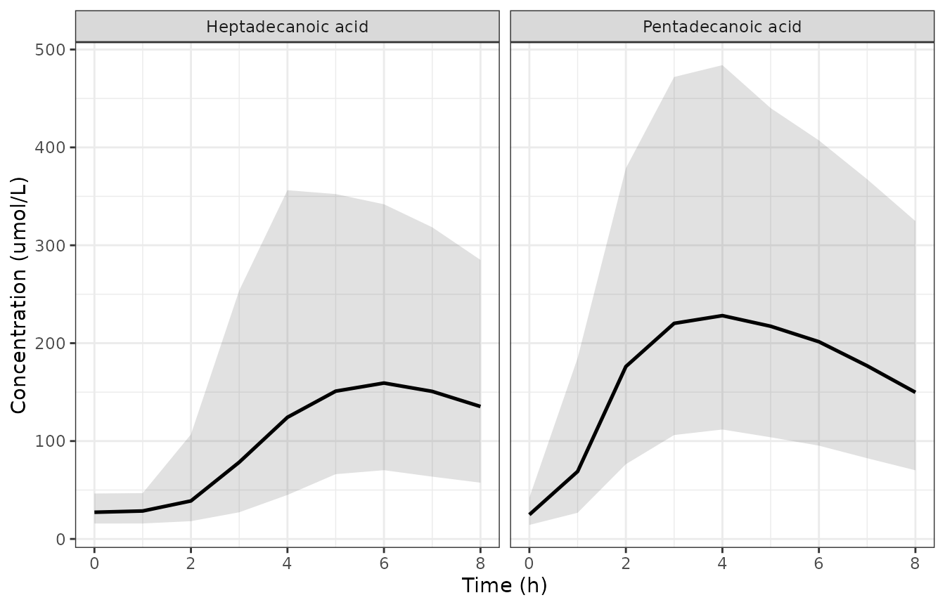
Replicates Figure 2 of Mascarenhas 2015 (visual predictive check, healthy subjects).
Medians read off the published Figure 2 alongside the simulated medians:
fig2_published <- tibble::tribble(
  ~analyte,              ~time, ~published,
  "Pentadecanoic acid",  0,  25, "Pentadecanoic acid", 1,  65,
  "Pentadecanoic acid",  2, 150, "Pentadecanoic acid", 3, 215,
  "Pentadecanoic acid",  4, 235, "Pentadecanoic acid", 5, 232,
  "Pentadecanoic acid",  6, 215, "Pentadecanoic acid", 7, 185,
  "Pentadecanoic acid",  8, 165,
  "Heptadecanoic acid",  0,  28, "Heptadecanoic acid", 1,  25,
  "Heptadecanoic acid",  2,  42, "Heptadecanoic acid", 3,  78,
  "Heptadecanoic acid",  4, 125, "Heptadecanoic acid", 5, 150,
  "Heptadecanoic acid",  6, 160, "Heptadecanoic acid", 7, 150,
  "Heptadecanoic acid",  8, 130
)

fig2_chk <- vpc %>%
  dplyr::filter(arm == "Healthy") %>%
  dplyr::inner_join(fig2_published, by = c("analyte", "time")) %>%
  dplyr::mutate(pct_diff = 100 * (median - published) / published)

knitr::kable(
  fig2_chk %>%
    dplyr::select(analyte, time, median, published, pct_diff) %>%
    dplyr::rename("Analyte" = analyte, "Time (h)" = time,
                  "Simulated median" = median, "Read from Figure 2" = published,
                  "Difference (%)" = pct_diff),
  digits = 1,
  caption = "Simulated versus published Figure 2 medians (healthy subjects)."
)| Analyte | Time (h) | Simulated median | Read from Figure 2 | Difference (%) |
|---|---|---|---|---|
| Heptadecanoic acid | 0 | 28.7 | 28 | 2.5 |
| Heptadecanoic acid | 1 | 29.2 | 25 | 16.8 |
| Heptadecanoic acid | 2 | 39.0 | 42 | -7.2 |
| Heptadecanoic acid | 3 | 79.1 | 78 | 1.4 |
| Heptadecanoic acid | 4 | 137.6 | 125 | 10.1 |
| Heptadecanoic acid | 5 | 172.8 | 150 | 15.2 |
| Heptadecanoic acid | 6 | 171.7 | 160 | 7.3 |
| Heptadecanoic acid | 7 | 161.3 | 150 | 7.5 |
| Heptadecanoic acid | 8 | 139.0 | 130 | 7.0 |
| Pentadecanoic acid | 0 | 26.1 | 25 | 4.4 |
| Pentadecanoic acid | 1 | 64.0 | 65 | -1.5 |
| Pentadecanoic acid | 2 | 175.8 | 150 | 17.2 |
| Pentadecanoic acid | 3 | 234.9 | 215 | 9.3 |
| Pentadecanoic acid | 4 | 246.8 | 235 | 5.0 |
| Pentadecanoic acid | 5 | 234.7 | 232 | 1.2 |
| Pentadecanoic acid | 6 | 210.5 | 215 | -2.1 |
| Pentadecanoic acid | 7 | 186.4 | 185 | 0.7 |
| Pentadecanoic acid | 8 | 165.9 | 165 | 0.6 |
These two sides differ by a physical mechanism that varies per subject (the transit-chain absorption lag, which decides how much of each analyte has been absorbed at any given hour), and the published side is a hand-digitised reading of a printed line. The assertion is therefore on the centre and a robust quantile rather than on the extreme:
Figure 3 – CF subjects taking enzymes with the MBT
ggplot(vpc %>% dplyr::filter(arm == "CF, enzymes with MBT"),
       aes(time, median)) +
  geom_ribbon(aes(ymin = p5, ymax = p95), alpha = 0.15) +
  geom_line(linewidth = 0.9) +
  facet_wrap(~analyte) +
  labs(x = "Time (h)", y = "Concentration (umol/L)") +
  theme_bw()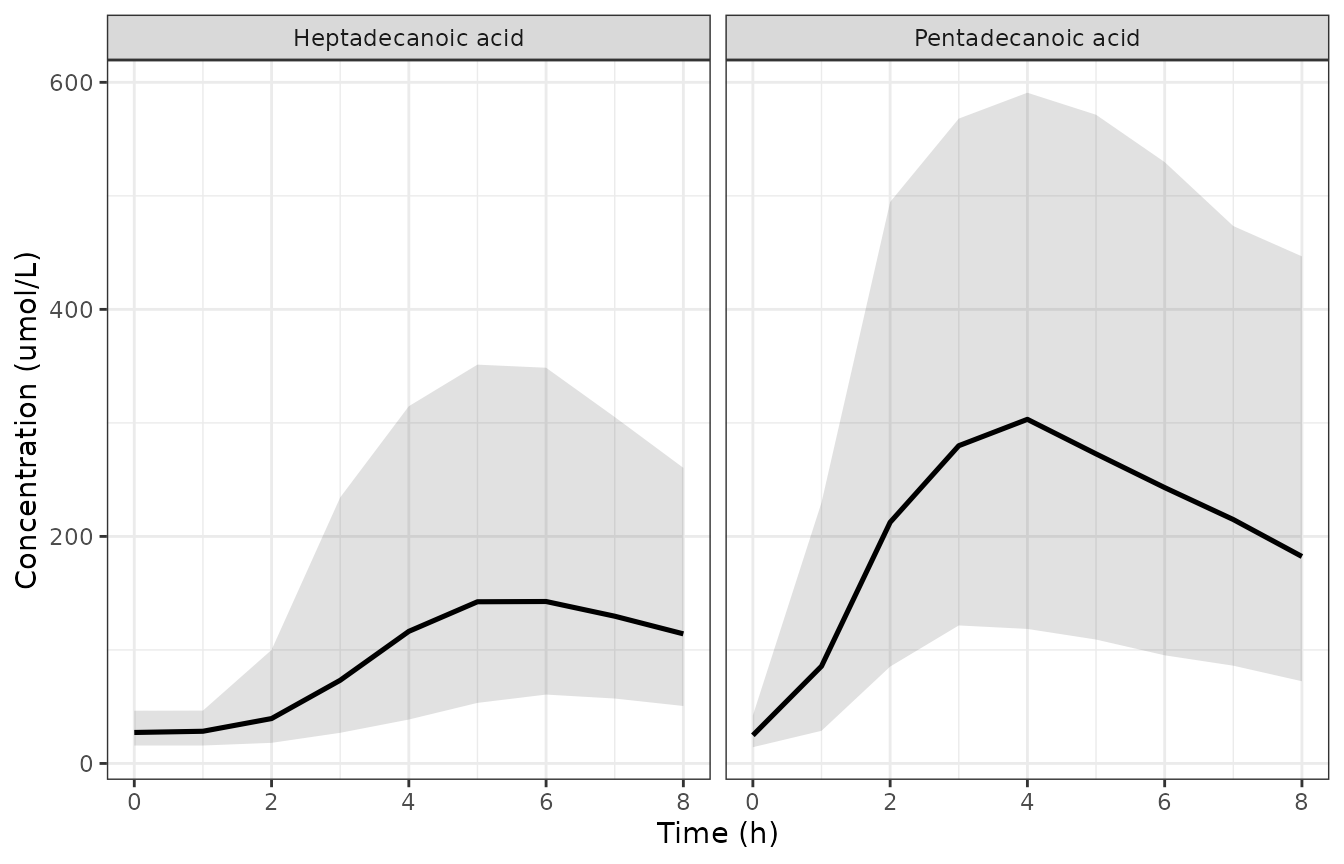
Replicates Figure 3 of Mascarenhas 2015 (CF subjects, enzymes with the MBT).
f3 <- vpc %>% dplyr::filter(arm == "CF, enzymes with MBT")
peak <- function(a) max(f3$median[f3$analyte == a])
# Read from Figure 3: PA median peaks near 290 umol/L, HA near 150 umol/L.
stopifnot(abs(peak("Pentadecanoic acid") - 290) / 290 < 0.15,
          abs(peak("Heptadecanoic acid") - 150) / 150 < 0.15)
c(PA_peak = peak("Pentadecanoic acid"), HA_peak = peak("Heptadecanoic acid"))
#>  PA_peak  HA_peak
#> 294.8472 143.1934
Figure 4 – CF subjects, varying enzyme timing
timing_order <- c("CF, enzymes -30 min", "CF, enzymes with MBT",
                  "CF, enzymes +30 min", "CF, enzymes +60 min")
ggplot(vpc %>% dplyr::filter(arm %in% timing_order) %>%
         dplyr::mutate(arm = factor(arm, levels = timing_order)),
       aes(time, median, colour = arm)) +
  geom_line(linewidth = 0.9) +
  facet_wrap(~analyte) +
  labs(x = "Time (h)", y = "Concentration (umol/L)", colour = NULL) +
  theme_bw() + theme(legend.position = "bottom")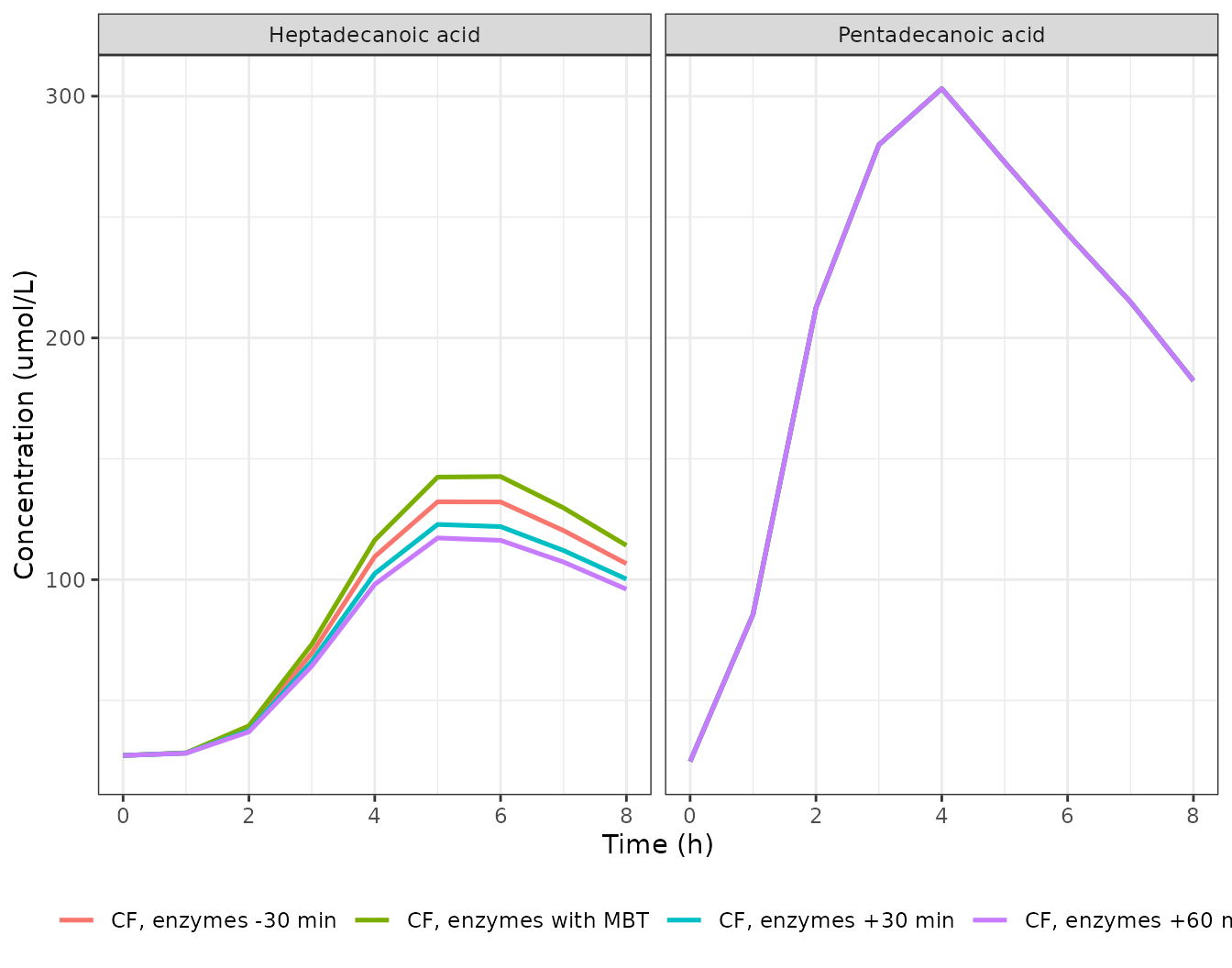
Replicates Figure 4 of Mascarenhas 2015 (CF subjects, enzymes at varying times relative to the MBT).
Figure 4 is plotted on a 0-1500 umol/L axis, so its median lines cannot be digitised to better than roughly 50 umol/L. What it does show unambiguously is that the pentadecanoic-acid medians are visually indistinguishable across the four timing panels while the heptadecanoic-acid medians fall as the enzyme dose is delayed. That qualitative claim is what is asserted:
peaks <- vpc %>%
  dplyr::filter(arm %in% timing_order) %>%
  dplyr::group_by(arm, analyte) %>%
  dplyr::summarise(peak = max(median), .groups = "drop") %>%
  tidyr::pivot_wider(names_from = analyte, values_from = peak)

knitr::kable(peaks %>% dplyr::rename("Arm" = arm), digits = 1,
caption = "Peak median concentration by enzyme-timing arm.")| Arm | Heptadecanoic acid | Pentadecanoic acid |
|---|---|---|
| CF, enzymes +30 min | 123.0 | 294.8 |
| CF, enzymes +60 min | 117.1 | 294.8 |
| CF, enzymes -30 min | 132.8 | 294.8 |
| CF, enzymes with MBT | 143.2 | 294.8 |
# PA peaks are flat across timing arms (spread < 1% of the mean).
pa_peaks <- peaks$`Pentadecanoic acid`
stopifnot(diff(range(pa_peaks)) / mean(pa_peaks) < 0.01)

# HA peaks decline monotonically as the enzyme dose is delayed.
ha_peaks <- peaks$`Heptadecanoic acid`[match(timing_order, peaks$arm)]
stopifnot(all(diff(ha_peaks[2:4]) < 0), ha_peaks[1] < ha_peaks[2])
Assumptions and deviations
- Figure 2 was reproduced at the final MBT dose, not the documented dose mixture. Table 1 states that the 27 healthy subjects were dosed in two groups: 15 received 2.5 g PA + 8.0 g THA (Orlistat Protocol) and 12 received 5.0 g PA + 5.5 g THA (Timing Protocol). Simulating that documented mixture reproduces neither analyte – the pentadecanoic-acid median peak comes out near 169 umol/L against roughly 235 read from the figure (28% low) while the heptadecanoic-acid peak comes out near 199 against roughly 160 (24% high). Being wrong in opposite directions for the two analytes is the signature of a dose-composition mismatch rather than a parameter error, because the two analytes’ doses move in opposite directions between the two protocols (PA 2.5 -> 5.0 g while THA 8.0 -> 5.5 g). Simulating all 27 healthy subjects at the final selected MBT dose of 5.0 g PA + 5.5 g THA matches both analytes simultaneously, to within 7% at every hour except t = 2 h. The most likely explanation is that the published figure was simulated at the dose the paper went on to select rather than at each subject’s own protocol dose. This is a property of the published figure, not of the model: the parameters in Table 2 are unaffected, and the exposure-ratio checks above – which are the paper’s actual claims – are dose-independent and pass exactly.
-
Heptadecanoic acid carries its own between-occasion
transit-time random effect. The typeset equation block on page
858 prints
eta_PA,IOV,MTTin both the PA and the HA mean-transit-time rows. That is a typesetting error, not a shared eta: Table 2 reports two distinct MTT intraindividual variances (0.205 and 0.102) with distinct confidence intervals, and the Results text states that between-occasion variability in MTT “was estimated to be 45.3% and 31.9% … for PA and HA, respectively”. The model implements two separate etas. -
The bioavailability between-occasion effect applies only to
the enzyme-treated CF arm. Table 2 parks the BOV percentages on
the
F_CFrow, but both the equation block (which placeseta_IOV,FonF_CF+Enzonly) and the Methods text (“Random effects for between-occasion variability in absorption mean transit time and bioavailability for CF subjects with administration of enzymes were also included”) put it on the enzyme branch. The prose and the equation are followed over the table’s row placement. -
The fasting baseline is an additive offset, not a decaying
initial condition. The paper says only that baseline
concentrations “were also estimated to account for variability in
concentration of fats at baseline”. The alternative reading –
central(0) = C0 x V, decaying atkel– is falsified by Figure 2: withkelfor heptadecanoic acid equal to 16.3 / 14.3 = 1.14 /h, a decaying initial condition would fall from 27.4 to about 8.8 umol/L within the first hour, whereas the published median is flat at roughly 28 umol/L from t = 0 to t = 1 h. These are endogenous fatty acids under continuous turnover, so a constant offset is also the physiologically sensible reading. -
Between-occasion variability is encoded as an
occasion-indicator expansion. rxode2 parses the
eta ~ var | occmulti-level syntax but cannot simulate from it, so each analyte’s MTT and bioavailability IOV is written as four per-occasion etas multiplexed byoc1..oc4, with occasions 2-4 fixed to the occasion-1 magnitude (the NONMEM$OMEGA BLOCK(1) SAMEidiom). This emits a benign “some etas defaulted to non-mu referenced” warning at parse time, which affects estimation only, not simulation. -
Age is documented but not implemented. The paper
screened a power age effect on CL/F for both analytes post hoc and did
not retain it: the exponent confidence intervals span zero and adding
the terms produced no drop in objective function value. It is recorded
in
covariatesDataExcludedso the provenance of the screen is preserved without declaring an unused covariate. -
Healthy subjects are the bioavailability reference and are
not estimated. F = 1 for both analytes when
DIS_CF = 0; all CF bioavailabilities are relative to that reference, as the paper states. -
The enzyme-dose covariate is binary, not
continuous. CF subjects took 4-7 Creon 20 capsules (80 000-140
000 lipase units). The paper reports that doses above the 80 000-unit
standard produced no increase in bioavailability, so
CONMED_PANCRELIPASEis encoded as a binary indicator. - The arms are simulated with common random numbers, and the enzyme-timing checks are paired rather than median-based. The three timing factors are only 6-17% apart, which is the same order as the Monte Carlo noise on a median over 200 independently drawn subjects – so an unpaired “medians must be monotone across the timing arms” assertion is not a real test, and would pass or fail depending on the rxode2 build that drew the cohort. Reseeding before each arm’s solve instead gives subject i the same random effects in every arm; because bioavailability multiplies the absorption input of a linear system, each subject’s own AUC ratio between two arms is then exactly the ratio of their bioavailabilities. The vignette asserts that per-subject identity to 1e-4, which is both far sharper and build-independent. Only the three widely-separated lipase-availability tiers (no enzymes / enzymes / healthy) are checked as an ordering of medians.
- Weight distributions are reconstructed. Table 1 reports cohort means, standard deviations, medians and ranges but not individual weights, so the virtual cohort draws truncated normals matched to the reported means and standard deviations and clipped to the reported ranges.