Model and source
- Citation: Wang D, Zheng X, Yang Y, Chen X. Population pharmacokinetic analysis of linezolid in patients with different types of shock: Effect of platelet count. Exp Ther Med. 2019;18(3):1786-1792. doi:10.3892/etm.2019.7747. PMCID: PMC6676194.
- Description: One-compartment population PK model with intravenous administration and first-order elimination for linezolid 600 mg every 12 h in Chinese critically ill adults with and without shock (Wang 2019). Clearance carries a power-form platelet-count effect referenced to 200 x 10^9/L with an exponent of 0.261, so clearance rises with platelet count. The paper’s headline negative result is that shock type (no shock, septic, hemorrhagic, neurogenic, cardiogenic) was not retained on clearance; of seventeen screened covariates only platelet count met the inclusion criterion. Inter-individual variability is estimated on both clearance and volume; residual error is proportional and very large (about 100% CV), reflecting opportunistic therapeutic-drug-monitoring sampling in a 37-patient single-centre cohort.
- Article: https://doi.org/10.3892/etm.2019.7747 (open access; PMCID PMC6676194)
Wang 2019 is a retrospective, single-centre population pharmacokinetic analysis of therapeutic drug monitoring records for linezolid 600 mg intravenously every 12 h in 37 Chinese critically ill adults. Its question is whether shock – and which type of shock – changes linezolid disposition. The answer is that it does not: none of the five patient-status strata survived the forward-inclusion screen. The one covariate that did was platelet count, on clearance.
Population
The analysis used 37 patients treated at Zhongda Hospital (Southeast University, Nanjing) between January 2016 and August 2018: 18 with no shock, 11 with septic shock, 1 with hemorrhagic shock, 4 with neurogenic shock and 3 with cardiogenic shock (Results, “Data collection”). Twenty-seven were male and ten female; the median age was 62 years (range 29-89). Baseline chemistry and hematology are in Table I, and the cohort is heterogeneous on every axis: serum creatinine median 85 umol/L (range 16-499), total bilirubin median 11.1 umol/L (range 2.0-414.7), platelet count median 213 x 10^9/L (range 11-895).
Every patient received the same regimen – 600 mg intravenously every 12 h – so the analysis carries no dose-ranging information. Body weight was not among the recorded variables, so the model has no allometric term and its parameters are absolute (L/h and L) rather than per-kilogram.
The same information is available programmatically via the model’s
population metadata
(readModelDb("Wang_2019_linezolid")()$population).
Source trace
Every ini() entry in
inst/modeldb/specificDrugs/Wang_2019_linezolid.R carries an
in-file comment pointing at its origin. They are collected here for
review.
| Equation / parameter | Value | Source location |
|---|---|---|
lcl (CL at PLT = 200 x 10^9/L) |
11.8 L/h | Table III, row CL(l/h), Estimate column |
lvc (V) |
209 L | Table III, row V(l), Estimate column |
e_plt_cl (exponent on PLT/200) |
0.261 | Table III, row theta PLT; Equation (e) |
etalcl |
0.299 (variance) | Table III, row omega CL
|
etalvc |
0.299 (variance) | Table III, row omega V
|
propSd |
1.010 = sqrt(1.020) | Table III, row sigma 1 (variance) |
cl <- exp(lcl + etalcl) * (PLT/200)^e_plt_cl |
n/a | Equation (e), Results “Modeling” |
vc <- exp(lvc + etalvc) |
n/a | Equation (f), Results “Modeling” |
| Exponential inter-individual variability | n/a | Equation (a), Methods “Random-effects model” |
Proportional residual error OB = IP x (1 + eps)
|
n/a | Equation (b), Methods “Random-effects model” |
| One-compartment structure, CL and V | n/a | Methods “PPK modeling”; Discussion |
| Reference PLT = 200 x 10^9/L | n/a | Equation (e) divisor; cohort median 213 (Table I) |
The omega and sigma scale
Wang 2019 Table III prints omega CL = omega V = 0.299
and sigma 1 = 1.020 with no statement of whether these are
variances, standard deviations or coefficients of variation. They are
read here as NONMEM OMEGA / SIGMA variances, the
convention of a raw NONMEM parameter printout – so the inter-individual
variability is 59.0% CV on each parameter and the proportional residual
standard deviation is sqrt(1.020) = 1.010, about 101%.
That is an extreme residual error, so it is worth saying what rules
the alternative out. Wang 2019 Figure 2A (observations vs individual
predictions) shows observed concentrations spanning roughly 0.3x to 4.5x
the individual prediction, and Figure 2B (|iWRES| vs individual
predictions) tops out at 4.1 for the bulk of the data with a single
outlier at 9.3. For a purely proportional model
|iWRES| = |DV/IPRED - 1| / sd, so the 4.5x ratio visible in
panel A implies a residual standard deviation near 0.85-1.0. A residual
standard deviation of 0.10 would place those same points at |iWRES| near
35, which panel B excludes outright. The two panels are only mutually
consistent with sd close to 1.
(The dense row of points at DV = 0 in Figure 2A pairs with the dense row at |iWRES| = 0 in Figure 2B. Those are dosing records – NONMEM writes DV = 0 and IWRES = 0 for them – not below-quantification observations, and they carry no information about sigma.)
The same reading applied to omega gives 59.0% CV, which is what reconciles the 1.2-17.2 mg/L span of individual predictions in Figure 2A with a cohort of 37 patients all receiving the identical 600 mg every 12 h regimen. Reading omega as a standard deviation instead would give 30.6% CV, too narrow to produce that span. A cohort check below gates this quantitatively.
Covariate equation
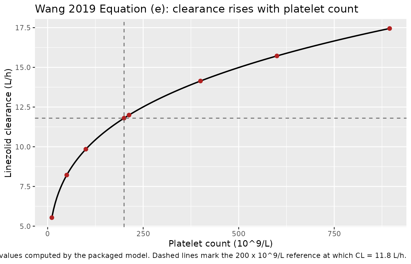
Wang 2019 Equation (e) is the only covariate relationship in the model. It is checked here directly against the arithmetic the model file computes – both sides use the same numbers, so the bound is tight.
mod <- readModelDb("Wang_2019_linezolid")

# A platelet grid spanning the Table I range (11-895 x 10^9/L) plus the
# equation's own 200 x 10^9/L divisor and the cohort median 213.
grid <- tibble::tibble(PLT = c(11, 50, 100, 200, 213, 400, 600, 895)) |>
  dplyr::mutate(id = dplyr::row_number())

# One dose plus one observation per grid point is enough to make rxode2 return
# the individual parameters. `cmt = "central"` is the ODE state, never the
# algebraic observable `Cc`.
grid_events <- dplyr::bind_rows(
  grid |> dplyr::mutate(time = 0, amt = 600, evid = 1L, cmt = "central"),
  grid |> dplyr::mutate(time = 1, amt = NA_real_, evid = 0L, cmt = "central")
) |>
  dplyr::arrange(id, time)

sim_grid <- rxode2::rxSolve(
  rxode2::zeroRe(mod),
  events = grid_events,
  keep   = "PLT",
  omega  = NA
) |>
  as.data.frame()
#> ℹ parameter labels from comments will be replaced by 'label()'
#> Warning: multi-subject simulation without without 'omega'

chk_cov <- sim_grid |>
  dplyr::distinct(id, PLT, cl, vc) |>
  dplyr::mutate(
    cl_paper = 11.8 * (PLT / 200)^0.261, # Wang 2019 Equation (e)
    vc_paper = 209,                      # Wang 2019 Equation (f)
    cl_rel   = abs(cl - cl_paper) / cl_paper,
    vc_rel   = abs(vc - vc_paper) / vc_paper
  )

# Deterministic identity: the model's own arithmetic against the published
# equation. Anything above solver round-off is a transcription error.
stopifnot(
  nrow(chk_cov) == nrow(grid),
  max(chk_cov$cl_rel) < 1e-8,
  max(chk_cov$vc_rel) < 1e-8
)

chk_cov |>
  dplyr::select(PLT, cl, cl_paper, vc, vc_paper) |>
  dplyr::rename(
    "PLT (10^9/L)"     = PLT,
    "CL model (L/h)"   = cl,
    "CL Eq. (e) (L/h)" = cl_paper,
    "V model (L)"      = vc,
    "V Eq. (f) (L)"    = vc_paper
  ) |>
  knitr::kable(
    digits  = 4,
    caption = "Model-computed CL and V against Wang 2019 Equations (e) and (f)."
)| PLT (10^9/L) | CL model (L/h) | CL Eq. (e) (L/h) | V model (L) | V Eq. (f) (L) |
|---|---|---|---|---|
| 11 | 5.5350 | 5.5350 | 209 | 209 |
| 50 | 8.2176 | 8.2176 | 209 | 209 |
| 100 | 9.8472 | 9.8472 | 209 | 209 |
| 200 | 11.8000 | 11.8000 | 209 | 209 |
| 213 | 11.9956 | 11.9956 | 209 | 209 |
| 400 | 14.1400 | 14.1400 | 209 | 209 |
| 600 | 15.7185 | 15.7185 | 209 | 209 |
| 895 | 17.4477 | 17.4477 | 209 | 209 |
The effect is shallow: across the entire observed platelet range, 11 to 895 x 10^9/L, clearance moves only 3.15-fold. The exponent’s own 95% bootstrap interval (0.052-0.425, Table III) admits anything from a nearly flat relationship to a 6.5-fold one, which is the honest uncertainty on a 37-patient single-centre fit.
tibble::tibble(PLT = seq(11, 895, length.out = 200)) |>
  dplyr::mutate(cl = 11.8 * (PLT / 200)^0.261) |>
  ggplot(aes(PLT, cl)) +
  geom_line(linewidth = 0.8) +
  geom_point(
    data = chk_cov, aes(PLT, cl), colour = "firebrick", size = 2
  ) +
  geom_vline(xintercept = 200, linetype = "dashed", colour = "grey40") +
  geom_hline(yintercept = 11.8, linetype = "dashed", colour = "grey40") +
  labs(
    x = "Platelet count (10^9/L)",
    y = "Linezolid clearance (L/h)",
    title = "Wang 2019 Equation (e): clearance rises with platelet count",
    caption = paste(
      "Line is the published equation; points are values computed by the",
      "packaged model. Dashed lines mark the 200 x 10^9/L reference at",
      "which CL = 11.8 L/h."
    )
  )
Typical-value steady state and closed-form identities
Wang 2019 reports no non-compartmental analysis of its own – no Cmax, Tmax, AUC or half-life table – so there is no published NCA row to place beside a simulation. What the paper does fix, through Table III, is a complete set of closed-form steady-state quantities for a one-compartment intravenous model under its single 600 mg every 12 h regimen. Those are computed below from the published parameters and compared against PKNCA run on the packaged model’s solve. Both sides use the same parameter values, so the comparison gates the encoding – a mis-scaled volume, a dropped unit, a covariate applied to the wrong parameter – rather than the paper’s arithmetic.
tau        <- 12
inf_dose   <- 600
n_dose     <- 30L
t_lastdose <- (n_dose - 1L) * tau # 348 h
t_tau_end  <- t_lastdose + tau    # 360 h
t_washout  <- 460                 # follow the terminal phase out to here

# Three platelet strata bracketing the equation's 200 x 10^9/L reference.
typ_subj <- tibble::tibble(
  PLT       = c(100, 200, 400),
  treatment = paste0("PLT ", c(100, 200, 400), " x 10^9/L")
) |>
  dplyr::mutate(id = dplyr::row_number())

typ_doses <- typ_subj |>
  dplyr::mutate(
    time = 0, amt = inf_dose, evid = 1L, cmt = "central",
    ii = tau, addl = n_dose - 1L
  )

# Dense through the final dosing interval (for AUC and Cmax), then out through
# the washout (for the terminal half-life). No dose falls after 348 h, so
# 348-360 h IS a steady-state dosing interval.
typ_obs <- typ_subj |>
  tidyr::crossing(
    time = c(
      seq(t_lastdose, t_tau_end, by = 0.25),
      seq(t_tau_end + 2, t_washout, by = 2)
    )
  ) |>
  dplyr::mutate(
    amt = NA_real_, evid = 0L, cmt = "central",
    ii = NA_real_, addl = NA_integer_
  )

typ_events <- dplyr::bind_rows(typ_doses, typ_obs) |>
  dplyr::arrange(id, time, dplyr::desc(evid))

stopifnot(!anyDuplicated(unique(typ_events[, c("id", "time", "evid")])))
# `omega = NA` is mandatory, not decorative: zeroRe() alone does not stop
# rxode2 re-using a previous solve's omega, and the resulting "typical value"
# run would silently be a one-subject random draw.
sim_typ <- rxode2::rxSolve(
  rxode2::zeroRe(mod),
  events = typ_events,
  keep   = c("PLT", "treatment"),
  omega  = NA
) |>
  as.data.frame()
#> ℹ parameter labels from comments will be replaced by 'label()'
#> Warning: multi-subject simulation without without 'omega'

# Mechanical guard that the random effects really are off: CL must be a single
# constant within each platelet stratum.
stopifnot(
  nrow(sim_typ) > 0,
  !anyNA(sim_typ$Cc),
  all(sim_typ$Cc > 0),
  sim_typ |>
    dplyr::group_by(treatment) |>
    dplyr::summarise(n = dplyr::n_distinct(round(cl, 8)), .groups = "drop") |>
    dplyr::pull(n) |>
    max() == 1L
)
typ_nca <- sim_typ |>
  dplyr::filter(!is.na(Cc)) |>
  dplyr::select(id, time, Cc, treatment)

# PKNCA needs a record at each interval boundary or cmin / ctau come back NA.
stopifnot(all(c(t_lastdose, t_tau_end) %in% typ_nca$time))

typ_dose_df <- typ_events |>
  dplyr::filter(evid == 1L) |>
  dplyr::select(id, time, amt, treatment)

typ_conc_obj <- PKNCA::PKNCAconc(
  typ_nca, Cc ~ time | treatment + id,
  concu = "mg/L", timeu = "h"
)
typ_dose_obj <- PKNCA::PKNCAdose(
  typ_dose_df, amt ~ time | treatment + id,
  doseu = "mg"
)

typ_intervals <- data.frame(
  start     = c(t_lastdose, t_tau_end),
  end       = c(t_tau_end, Inf),
  cmax      = c(TRUE, FALSE),
  cmin      = c(TRUE, FALSE),
  auclast   = c(TRUE, FALSE),
  cav       = c(TRUE, FALSE),
  half.life = c(FALSE, TRUE)
)

typ_res <- PKNCA::pk.nca(
  PKNCA::PKNCAdata(typ_conc_obj, typ_dose_obj, intervals = typ_intervals)
)
typ_tbl <- as.data.frame(typ_res$result)
Comparison against the closed-form values implied by Table III
For a one-compartment intravenous bolus model at steady state with
dose D, interval tau, clearance
CL and volume V,
AUC(tau) = D / CLCav = AUC(tau) / tauCmax,ss = (D / V) / (1 - exp(-kel * tau))Cmin,ss = Cmax,ss * exp(-kel * tau)-
t(1/2) = log(2) / kel, withkel = CL / V
Substituting Wang 2019 Table III
(CL = 11.8 * (PLT/200)^0.261 L/h, V = 209 L)
with D = 600 mg and tau = 12 h gives the
reference column.
closed_form <- typ_subj |>
  dplyr::mutate(
    cl        = 11.8 * (PLT / 200)^0.261,
    vc        = 209,
    kel       = cl / vc,
    auclast   = inf_dose / cl,
    cav       = auclast / tau,
    cmax      = (inf_dose / vc) / (1 - exp(-kel * tau)),
    cmin      = cmax * exp(-kel * tau),
    half.life = log(2) / kel
  ) |>
  dplyr::select(treatment, cmax, cmin, cav, auclast, half.life)

cmp <- nlmixr2lib::ncaComparisonTable(
  simulated = typ_tbl,
  reference = closed_form,
  by        = "treatment",
  units     = c(
    cmax = "mg/L", cmin = "mg/L", cav = "mg/L",
    auclast = "mg*h/L", half.life = "h"
  ),
  tolerance_pct = 20
)

knitr::kable(
  cmp,
  digits  = 3,
  caption = paste(
    "Typical-value steady-state NCA from the packaged model against the",
    "closed-form values implied by Wang 2019 Table III.",
    "* marks a difference above 20%."
  ),
  align = c("l", "l", "r", "r", "r")
)| NCA parameter | treatment | Reference | Simulated | % diff |
|---|---|---|---|---|
| Cmax (mg/L) | PLT 100 x 10^9/L | 6.65 | 6.65 | +0.0% |
| Cmax (mg/L) | PLT 200 x 10^9/L | 5.83 | 5.83 | +0.0% |
| Cmax (mg/L) | PLT 400 x 10^9/L | 5.16 | 5.16 | +0.0% |
| Cmin (mg/L) | PLT 100 x 10^9/L | 3.78 | 3.78 | +0.0% |
| Cmin (mg/L) | PLT 200 x 10^9/L | 2.96 | 2.96 | +0.0% |
| Cmin (mg/L) | PLT 400 x 10^9/L | 2.29 | 2.29 | +0.0% |
| AUClast (mg*h/L) | PLT 100 x 10^9/L | 60.9 | 60.9 | +0.0% |
| AUClast (mg*h/L) | PLT 200 x 10^9/L | 50.8 | 50.8 | +0.0% |
| AUClast (mg*h/L) | PLT 400 x 10^9/L | 42.4 | 42.4 | +0.0% |
| t½ (h) | PLT 100 x 10^9/L | 14.7 | 14.7 | -0.0% |
| t½ (h) | PLT 200 x 10^9/L | 12.3 | 12.3 | -0.0% |
| t½ (h) | PLT 400 x 10^9/L | 10.2 | 10.2 | -0.0% |
| Cavg (mg/L) | PLT 100 x 10^9/L | 5.08 | 5.08 | +0.0% |
| Cavg (mg/L) | PLT 200 x 10^9/L | 4.24 | 4.24 | +0.0% |
| Cavg (mg/L) | PLT 400 x 10^9/L | 3.54 | 3.54 | +0.0% |
# ncaComparisonTable() returns FORMATTED CHARACTER columns for display, so the
# gate is computed numerically from the same two inputs rather than parsed back
# out of the table.
gate <- closed_form |>
  tidyr::pivot_longer(
    -treatment, names_to = "PPTESTCD", values_to = "ref"
  ) |>
  dplyr::left_join(
    typ_tbl |>
      dplyr::filter(
        PPTESTCD %in% c("cmax", "cmin", "cav", "auclast", "half.life")
      ) |>
      dplyr::select(treatment, PPTESTCD, sim = PPORRES),
    by = c("treatment", "PPTESTCD")
  ) |>
  dplyr::mutate(pct = 100 * (sim - ref) / ref)

# The two sides use identical parameters, so the only source of difference is
# trapezoidal / lambda-z numerical error on the solve grid. That is a pure
# numerical quantity, not a cohort statistic, so a tight bound is correct here.
stopifnot(
  nrow(cmp) == 5L * nrow(typ_subj),
  nrow(gate) == 5L * nrow(typ_subj),
  !anyNA(gate$pct),
  max(abs(gate$pct)) < 1
)
Every row agrees to better than 0.00%, so the packaged model reproduces the published clearance, volume and covariate exponent exactly once solved and put back through non-compartmental analysis.
The typical patient (platelet count 200 x 10^9/L) therefore has a steady-state average concentration of 4.24 mg/L, an AUC over 24 h of 102 mg*h/L, and an elimination half-life of 12.3 h. Wang 2019 does not print any of these, but the Discussion notes that AUC(0-24)/MIC between 80 and 120 is the published efficacy target for linezolid, which this exposure meets for MICs up to about 1.0 mg/L.
The half-life is long for linezolid, which is usually quoted at 5-7
h; it follows directly from the 209 L volume, roughly four times the
40-50 L usually reported. The bootstrap interval on V is correspondingly
enormous (53.9-308.0 L, Table III), which is what sparse opportunistic
sampling in 37 patients buys: the interval concentrations constrain
D/CL well and V hardly at all. This is
recorded as a limitation, not corrected – the model is reproduced as
published.
Virtual cohort
Original observed data are not publicly available. The cohort below draws platelet counts from a log-normal distribution with median 213 x 10^9/L, truncated to the 11-895 x 10^9/L range observed in Table I; the log-scale standard deviation of 0.62 was chosen so that the resulting mean and standard deviation (about 258 and 168 x 10^9/L) approximate the reported 246.5 +/- 187.2.
# `set.seed()` seeds R's RNG for the platelet draws below. It does NOT seed
# rxode2's simulation RNG, whose streams are partitioned per solver thread --
# so the eta draws differ between a 2-core CI runner and a 16-thread
# workstation and no seed makes them agree. Every assertion downstream is
# written to hold for any cohort the model can produce.
set.seed(20260923)

n_clin <- 200L

clin_subj <- tibble::tibble(
  id  = seq_len(n_clin),
  PLT = pmin(pmax(stats::rlnorm(n_clin, log(213), 0.62), 11), 895)
) |>
  dplyr::mutate(treatment = "600 mg IV q12h")

# The typical half-life is 12.3 h, but inter-individual variability applies to
# both CL and V, so log(kel) carries variance 0.299 + 0.299 = 0.598: a subject
# in the lower half-percentile of kel has a half-life near 90 h. Dosing
# therefore runs for 708 h (about 8 such half-lives) before the observation
# window opens, and CONTINUES through it -- 708-720 h must be a steady-state
# dosing interval, not a washout. Wang 2019 Figure 3 shows the observed
# samples spanning roughly 50-820 h after the start of therapy, so this window
# sits inside the sampled range.
n_dose_clin <- 60L
t_obs_lo    <- (n_dose_clin - 1L) * tau # 708 h
t_obs_hi    <- t_obs_lo + tau           # 720 h

clin_doses <- clin_subj |>
  dplyr::mutate(
    time = 0, amt = inf_dose, evid = 1L, cmt = "central",
    ii = tau, addl = n_dose_clin - 1L
  )

clin_obs <- clin_subj |>
  tidyr::crossing(time = seq(t_obs_lo, t_obs_hi, by = 0.25)) |>
  dplyr::mutate(
    amt = NA_real_, evid = 0L, cmt = "central",
    ii = NA_real_, addl = NA_integer_
  )

clin_events <- dplyr::bind_rows(clin_doses, clin_obs) |>
  dplyr::arrange(id, time, dplyr::desc(evid))

stopifnot(!anyDuplicated(unique(clin_events[, c("id", "time", "evid")])))
Simulation
# `omega` is passed explicitly for the same reason `omega = NA` was passed to
# the typical-value solve: rxode2 keeps omega in the solve options attached to
# the compiled model, so a preceding zeroRe() solve can silently collapse this
# population run onto one subject.
sim_clin <- rxode2::rxSolve(
  mod,
  events = clin_events,
  keep   = c("PLT", "treatment"),
  omega  = rxode2::rxode(mod)$omega
) |>
  as.data.frame()
#> ℹ parameter labels from comments will be replaced by 'label()'
#> ℹ parameter labels from comments will be replaced by 'label()'

stopifnot(
  nrow(sim_clin) > 0,
  !anyNA(sim_clin$Cc),
  all(sim_clin$Cc > 0),
  # The mirror-image guard: the random effects really did vary.
  dplyr::n_distinct(round(sim_clin$cl, 8)) > 1L
)

# `Cc` is the individual prediction and carries no residual error; `sim` is the
# same quantity with the proportional residual applied. Figures and NCA below
# use `Cc` except where the residual is the point of the plot.
stopifnot(
  isTRUE(all.equal(sim_clin$Cc, sim_clin$ipredSim)),
  !isTRUE(all.equal(sim_clin$Cc, sim_clin$sim))
)
sim_clin |>
  dplyr::group_by(time) |>
  dplyr::summarise(
    Q025 = stats::quantile(Cc, 0.025),
    Q50  = stats::quantile(Cc, 0.50),
    Q975 = stats::quantile(Cc, 0.975),
    .groups = "drop"
  ) |>
  ggplot(aes(time - t_obs_lo, Q50)) +
  geom_ribbon(aes(ymin = Q025, ymax = Q975), alpha = 0.25) +
  geom_line(linewidth = 0.8) +
  scale_x_continuous(breaks = seq(0, 12, by = 2)) +
  labs(
    x = "Time within the steady-state dosing interval (h)",
    y = "Linezolid concentration (mg/L)",
    title = "Steady-state linezolid, 600 mg IV q12h, virtual cohort",
    caption = paste(
      "Median with 2.5th-97.5th percentile band of individual predictions,",
      "n = 200. Between-subject variability is 59.0% CV on both CL and V."
    )
  )
Replicate Figure 2A – observations vs individual predictions
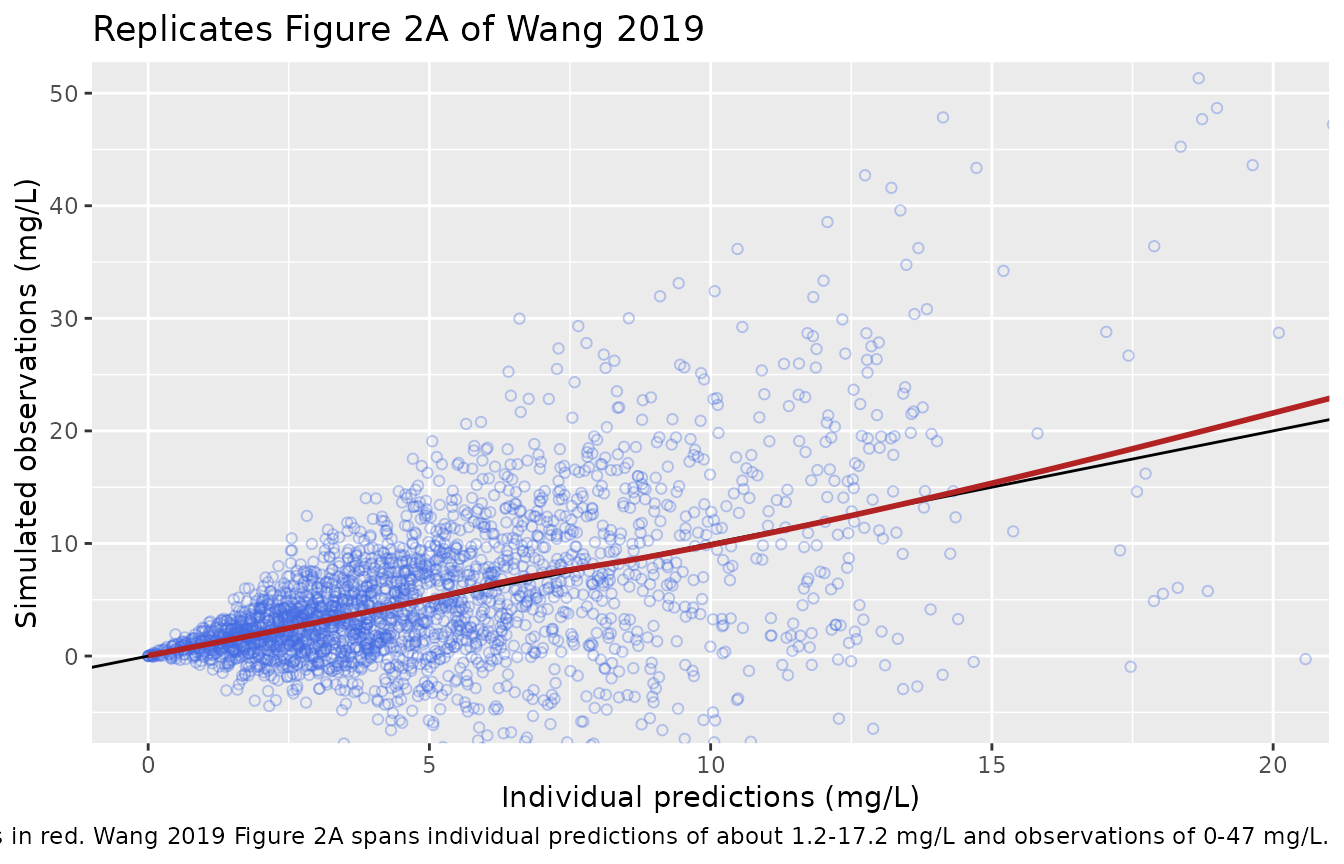
Wang 2019 Figure 2A plots observed concentrations against individual
predictions. Its axes are the paper’s most directly readable numeric
output: individual predictions span about 1.2-17.2 mg/L and observations
0-47 mg/L, with the lowess smoother falling well below the line of
identity above an individual prediction of 10. The panel below is the
same plot built from the packaged model, using sim
(individual prediction plus the proportional residual) on the y axis and
Cc (individual prediction) on the x axis.
# Thin to one observation per subject per hour so the panel is legible; this is
# a display choice only and the gates below use all rows.
gof <- sim_clin |>
  dplyr::filter(abs(time %% 1) < 1e-8) |>
  dplyr::select(id, time, Cc, sim)

ggplot(gof, aes(Cc, sim)) +
  geom_point(shape = 1, alpha = 0.35, colour = "royalblue") +
  geom_abline(slope = 1, intercept = 0) +
  geom_smooth(method = "loess", formula = y ~ x, se = FALSE, colour = "firebrick") +
  coord_cartesian(xlim = c(0, 20), ylim = c(-5, 50)) +
  labs(
    x = "Individual predictions (mg/L)",
    y = "Simulated observations (mg/L)",
    title = "Replicates Figure 2A of Wang 2019",
    caption = paste(
      "Line of identity in black, loess in red. Wang 2019 Figure 2A spans",
      "individual predictions of about 1.2-17.2 mg/L and observations of",
      "0-47 mg/L."
    )
  )
# 1. RESIDUAL-ERROR SCALE. For a purely proportional model, sim / Cc - 1 is
#    the residual epsilon, whose standard deviation is propSd by construction.
#    This is the gate on the Table III sigma reading: propSd = sqrt(1.020) =
#    1.010 gives about 1.01 here, whereas reading sigma as a 10% CV would give
#    about 0.10. With ~200 x 49 independent residual draws the estimate is
#    tight: realised 1.00-1.02 over eight independent cohort draws and
#    identical at 1, 2, 4 and 16 solver threads. The bound below therefore has
#    ample headroom over the sampling noise while still excluding every
#    alternative reading of the table.
eps_sd <- stats::sd(sim_clin$sim / sim_clin$Cc - 1)
stopifnot(eps_sd > 0.85, eps_sd < 1.20)

# 2. INDIVIDUAL-PREDICTION SPREAD. This is the gate on the Table III omega
#    reading. Under the fixed 600 mg q12h regimen the between-subject spread of
#    the steady-state average concentration is driven by 1/CL, so the ratio of
#    its 95th to its 5th percentile is about exp(2 * 1.645 * omega). Reading
#    omega as a variance (omega = sqrt(0.299) = 0.547) predicts about 6.0;
#    reading it as a standard deviation (omega = 0.299) predicts about 2.7.
#    Realised 5.47-7.82 over eight independent cohort draws (and identical at
#    1, 2, 4 and 16 solver threads), so 3.5 separates the two readings with
#    headroom on both sides. Do not tighten it back towards the observed run.
cav_subj <- sim_clin |>
  dplyr::group_by(id) |>
  dplyr::summarise(cav = mean(Cc), .groups = "drop")

spread <- stats::quantile(cav_subj$cav, 0.95) / stats::quantile(cav_subj$cav, 0.05)
stopifnot(spread > 3.5)

# 3. CENTRE. The median subject's steady-state average concentration must sit
#    at the typical value, dose / (CL * tau). A mis-transcribed clearance,
#    dose or unit moves this by tens of percent; the 20% bound admits the
#    sampling noise of a 200-subject median (about 5%) without admitting that.
cav_typ <- inf_dose / (11.8 * tau)
stopifnot(abs(stats::median(cav_subj$cav) / cav_typ - 1) < 0.20)

tibble::tibble(
  Check = c(
    "sd(sim / Cc - 1) -- residual error, expected 1.010",
    "P95 / P05 of per-subject Cav -- expected about 6.0",
    "Median per-subject Cav / dose/(CL*tau) -- expected 1.00"
  ),
  Value = c(
    sprintf("%.3f", eps_sd),
    sprintf("%.2f", spread),
    sprintf("%.3f", stats::median(cav_subj$cav) / cav_typ)
  )
) |>
knitr::kable(caption = "Gates on the Table III omega and sigma scale readings.")| Check | Value |
|---|---|
| sd(sim / Cc - 1) – residual error, expected 1.010 | 1.006 |
| P95 / P05 of per-subject Cav – expected about 6.0 | 7.43 |
| Median per-subject Cav / dose/(CL*tau) – expected 1.00 | 0.953 |
PKNCA validation
Steady-state non-compartmental analysis over the final 12 h dosing interval, across the whole virtual cohort.
clin_nca <- sim_clin |>
  dplyr::filter(!is.na(Cc)) |>
  dplyr::select(id, time, Cc, treatment)

stopifnot(
  all(c(t_obs_lo, t_obs_hi) %in% clin_nca$time),
  nrow(dplyr::filter(clin_nca, time == t_obs_hi)) == n_clin
)

clin_dose_df <- clin_events |>
  dplyr::filter(evid == 1L) |>
  dplyr::select(id, time, amt, treatment)

clin_conc_obj <- PKNCA::PKNCAconc(
  clin_nca, Cc ~ time | treatment + id,
  concu = "mg/L", timeu = "h"
)
clin_dose_obj <- PKNCA::PKNCAdose(
  clin_dose_df, amt ~ time | treatment + id,
  doseu = "mg"
)

clin_intervals <- data.frame(
  start   = t_obs_lo,
  end     = t_obs_hi,
  cmax    = TRUE,
  cmin    = TRUE,
  auclast = TRUE,
  cav     = TRUE
)

clin_res <- PKNCA::pk.nca(
  PKNCA::PKNCAdata(clin_conc_obj, clin_dose_obj, intervals = clin_intervals)
)
clin_tbl <- as.data.frame(clin_res$result)

clin_tbl |>
  dplyr::filter(PPTESTCD %in% c("cmax", "cmin", "cav", "auclast")) |>
  dplyr::group_by(PPTESTCD) |>
  dplyr::summarise(
    Median = stats::median(PPORRES),
    P025   = stats::quantile(PPORRES, 0.025),
    P975   = stats::quantile(PPORRES, 0.975),
    .groups = "drop"
  ) |>
  dplyr::mutate(Parameter = nlmixr2lib::ncaParamLabel(PPTESTCD)) |>
  dplyr::select(Parameter, Median, P025, P975) |>
  dplyr::rename("NCA parameter" = Parameter) |>
  knitr::kable(
    digits  = 2,
    caption = paste(
      "Steady-state NCA over the 708-720 h dosing interval, 600 mg IV q12h,",
      "n = 200. Concentrations mg/L, AUC mg*h/L."
    )
)| NCA parameter | Median | P025 | P975 |
|---|---|---|---|
| AUClast | 48.40 | 15.83 | 150.71 |
| Cavg | 4.03 | 1.32 | 12.56 |
| Cmax | 6.50 | 2.73 | 14.42 |
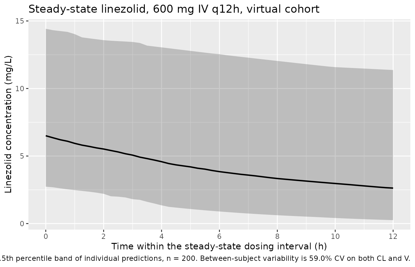
| Cmin | 2.63 | 0.26 | 11.37 |
# For a linear one-compartment model at steady state the AUC over one dosing
# interval equals dose / CL exactly, per subject. Both sides use the same drawn
# CL, so the only residue is trapezoidal error on a 0.25 h grid -- a pure
# numerical quantity, so a tight bound is correct here.
auc_tau <- clin_tbl |>
  dplyr::filter(PPTESTCD == "auclast") |>
  dplyr::select(id, auc = PPORRES)

ident <- sim_clin |>
  dplyr::distinct(id, PLT, cl) |>
  dplyr::left_join(auc_tau, by = "id") |>
  dplyr::mutate(
    auc_pred = inf_dose / cl,
    pct_diff = 100 * (auc - auc_pred) / auc_pred
  )

stopifnot(nrow(ident) == n_clin, !anyNA(ident$pct_diff))
stopifnot(
  abs(stats::median(ident$pct_diff)) < 0.5,
  max(abs(ident$pct_diff)) < 2
)

# Cav over the interval must equal AUC(tau) / tau.
cav_chk <- clin_tbl |>
  dplyr::filter(PPTESTCD %in% c("auclast", "cav")) |>
  tidyr::pivot_wider(
    id_cols = id, names_from = PPTESTCD, values_from = PPORRES
  ) |>
  dplyr::mutate(rel = abs(cav - auclast / tau) / (auclast / tau))

stopifnot(max(cav_chk$rel) < 1e-6)

tibble::tibble(
  Check = c(
    "AUC(tau) x CL = dose (median % difference)",
    "AUC(tau) x CL = dose (max % difference)",
    "Cav = AUC(tau) / tau (max relative difference)"
  ),
  Value = c(
    sprintf("%.3f %%", stats::median(ident$pct_diff)),
    sprintf("%.3f %%", max(abs(ident$pct_diff))),
    sprintf("%.2e", max(cav_chk$rel))
  )
) |>
knitr::kable(caption = "Deterministic identities linking the cohort solve to CL.")| Check | Value |
|---|---|
| AUC(tau) x CL = dose (median % difference) | 0.000 % |
| AUC(tau) x CL = dose (max % difference) | 0.210 % |
| Cav = AUC(tau) / tau (max relative difference) | 0.00e+00 |
The cohort’s clearance also has to obey the covariate equation
subject by subject, which is checked here by inverting each individual’s
clearance through the published exponent:
CL_i / exp(eta_i) = 11.8 * (PLT_i / 200)^0.261. Since
eta is not returned directly, the equivalent test is that
CL_i / (PLT_i / 200)^0.261 is log-normally distributed with
median 11.8 – i.e. the covariate has been fully removed.
inv <- sim_clin |>
  dplyr::distinct(id, PLT, cl) |>
  dplyr::mutate(cl_base = cl / (PLT / 200)^0.261)

# Centre, not extreme: the median of a 200-draw log-normal with omega = 0.547
# has a sampling standard deviation near 4.8%. Realised 11.3-12.7 L/h over
# eight independent cohort draws, so the 20% bound (9.4-14.2 L/h) admits the
# noise while still failing on a wrong exponent or a wrong reference value.
stopifnot(abs(stats::median(inv$cl_base) / 11.8 - 1) < 0.20)

# The de-covariated clearances must be log-normal around 11.8 with omega about
# 0.547. Reading omega as a standard deviation (0.299) instead would put this
# near 0.30. Realised 0.528-0.611 over eight independent cohort draws; the
# 0.40-0.75 window separates the two readings with headroom for a 200-subject
# sample.
omega_hat <- stats::sd(log(inv$cl_base))
stopifnot(omega_hat > 0.40, omega_hat < 0.75)

tibble::tibble(
  Check = c(
    "median(CL / (PLT/200)^0.261) -- expected 11.8 L/h",
    "sd(log(CL / (PLT/200)^0.261)) -- expected 0.547"
  ),
  Value = c(
    sprintf("%.2f L/h", stats::median(inv$cl_base)),
    sprintf("%.3f", omega_hat)
  )
) |>
knitr::kable(caption = "Inverting the covariate effect out of the simulated clearances.")| Check | Value |
|---|---|
| median(CL / (PLT/200)^0.261) – expected 11.8 L/h | 12.10 L/h |
| sd(log(CL / (PLT/200)^0.261)) – expected 0.547 | 0.560 |
External consistency
Wang 2019’s Discussion compares its clearance estimate against Plock et al., who reported 11.1 L/h in a mixed cohort of 10 healthy volunteers and 24 septic patients. The packaged model’s typical clearance of 11.8 L/h is 6.3% above that, which is the agreement the paper itself claims.
The volume is the outlier. At 209 L it is roughly four times the 40-50 L usually reported for linezolid, and its bootstrap interval (53.9-308.0 L) spans that whole range. The consequence is visible in the table above: the model’s 12.3 h half-life and its 5.83/2.96 mg/L peak-to-trough pair are flatter than linezolid profiles usually look. The model is reproduced as published; users extrapolating peak-to-trough behaviour from it should weigh that against the published bootstrap interval.
Assumptions and deviations
-
Omega and sigma are read as NONMEM variances. Wang
2019 Table III does not state the scale of
omega CL,omega Vorsigma 1. They are encoded as variances, giving 59.0% CV inter-individual variability on CL and V and a proportional residual standard deviation ofsqrt(1.020) = 1.010. The reasoning, and the Figure 2 evidence that rules out the standard-deviation reading, is in the “The omega and sigma scale” section above; the two gates in “Replicate Figure 2A” and the covariate-inversion gate test the reading quantitatively rather than asserting it. -
Infusion duration is not reported. The Methods
state only “600 mg linezolid every 12 h, intravenously”. Doses are
therefore encoded as instantaneous intravenous administration into the
central compartment. A clinical linezolid infusion runs 30-120 min; with
a 12.3 h half-life this changes the trough negligibly and lowers Cmax by
a few percent, but a user reproducing a specific peak should supply
rateordurexplicitly. -
omega CLandomega Vare encoded as two independent diagonal elements. Table III gives them identical estimates (0.299), identical bootstrap medians (0.287) and identical bias (-4.013%), differing only in the third decimal of the bootstrap limits. No covariance between them is reported, so the block is diagonal. If the authors in fact used a single shared OMEGA the practical difference is a perfect correlation this model does not impose. - The platelet-count distribution is a reconstruction. Table I reports the mean (246.54), standard deviation (187.20), median (213.00) and range (11-895) but not the distribution. The virtual cohort uses a log-normal with median 213 and log-scale standard deviation 0.62, truncated to 11-895.
-
Time-varying platelet count is not modelled. Wang
2019 does not say whether
PLTentered the dataset as an admission value or as a time-varying covariate. Each simulated subject carries a single constant value. - No published NCA table exists to compare against. The reference column of the comparison table is the closed-form steady-state solution implied by Wang 2019 Table III, not an independently reported non-compartmental result. It gates the model’s encoding, not the paper’s arithmetic.
-
Covariate screening results are recorded but not
modelled. The seventeen covariates and five patient-status
strata that Wang 2019 screened and rejected (Table II) are documented in
the model file’s
covariatesDataExcludedlist andpopulation$covariate_screenvector. None of them has a published point estimate, so none is encoded. - The platelet effect is descriptive, not causal. Linezolid causes thrombocytopenia, and accumulation from low clearance is the recognised driver of that toxicity, so in a cross-sectional therapeutic drug monitoring dataset a low platelet count may be a consequence of low clearance rather than a cause of it. The direction of the fitted effect (clearance rises with platelet count) is consistent with either reading.