Potassium homeostasis and spironolactone QSP (Meid 2024) • nlmixr2lib

Model and source

mod <- rxode2::rxode2(readModelDb("Meid_2024_spironolactone_qsp"))
#> ℹ parameter labels from comments will be replaced by 'label()'
meta <- readModelDb("Meid_2024_spironolactone_qsp")()

Citation: Meid AD, Scherkl C, Metzner M, Czock D, Seidling HM (2024). Real-World Application of a Quantitative Systems Pharmacology (QSP) Model to Predict Potassium Concentrations from Electronic Health Records: A Pilot Case towards Prescribing Monitoring of Spironolactone. Pharmaceuticals 17(8):1041. doi:10.3390/ph17081041. Structural model and physiological constants inherited from Maddah E, Hallow KM (2022), A quantitative systems pharmacology model of plasma potassium regulation by the kidney and aldosterone, J Pharmacokinet Pharmacodyn 49:471-486, doi:10.1007/s10928-022-09815-x; every value used here is taken from the Meid 2024 Appendix C listing, not from the upstream paper (which is not open access). Spironolactone / canrenone disposition traces to Gardiner 1989 (J Clin Pharmacol 29:342-347) as cited by Meid 2024 reference 15.
Article: https://doi.org/10.3390/ph17081041
Model source listing: Meid 2024 Appendix C (“Operationalized R code (rxode2 format transported from the RxODE code from the original QSP model developed by Maddah and Hallow 2022)”).

Meid 2024 is an application paper: it takes the Maddah and Hallow (2022) quantitative-systems-pharmacology model of plasma-potassium regulation and operationalizes it for prospective, Bayesian, per-patient prediction of potassium trajectories from hospital electronic health records. Its Appendix C prints the complete rxode2 model text – every ODE, every physiological constant, and every initial condition – so the model is fully reproducible from this paper alone. That is why this extraction does not depend on the (paywalled) upstream publication.

The model is deliberately not a pharmacokinetic model of spironolactone. Its observation variable is plasma potassium: Appendix C ends with Cc = plasma_K. Spironolactone and its active metabolite canrenone enter only as a pharmacological perturbation of the potassium-regulating system.

Structure

data.frame(
  state = mod$state,
  role = c(
    "spironolactone oral depot",
    "spironolactone absorption transit 1",
    "spironolactone absorption transit 2",
    "extracellular (plasma) potassium amount",
    "intracellular potassium amount",
    "DCT luminal potassium amount (single nephron)",
    "CNT luminal potassium amount (single nephron)",
    "CCD luminal potassium amount (single nephron)",
    "DCT principal-cell potassium concentration",
    "CNT principal-cell potassium concentration",
    "CCD principal-cell potassium concentration",
    "cumulative urinary potassium excretion",
    "fraction of mineralocorticoid receptor NOT inhibited",
    "spironolactone plasma concentration",
    "canrenone plasma concentration (central)",
    "canrenone plasma concentration (peripheral)"
  )
) |>
  dplyr::rename("ODE state" = state, "Role" = role) |>
  knitr::kable()

ODE state	Role
depot	spironolactone oral depot
transit1	spironolactone absorption transit 1
transit2	spironolactone absorption transit 2
k_ecf	extracellular (plasma) potassium amount
intracellular_k	intracellular potassium amount
dct_luminal_k_amount	DCT luminal potassium amount (single nephron)
cnt_luminal_k_amount	CNT luminal potassium amount (single nephron)
ccd_luminal_k_amount	CCD luminal potassium amount (single nephron)
dct_cell_k_conc	DCT principal-cell potassium concentration
cnt_cell_k_conc	CNT principal-cell potassium concentration
ccd_cell_k_conc	CCD principal-cell potassium concentration
potassium_excretion	cumulative urinary potassium excretion
mra_effect	fraction of mineralocorticoid receptor NOT inhibited
central	spironolactone plasma concentration
central_canrenone	canrenone plasma concentration (central)
peripheral1_canrenone	canrenone plasma concentration (peripheral)

Population

pop <- meta$population

The pilot validation sample is 9 hospitalised adults newly initiating spironolactone at Heidelberg University Hospital (a 2500-bed German tertiary-care centre), admitted between 1 January and 31 March 2023 (Meid 2024 Table A2). Age 56-88 years (mean 68, SD 12); weight 54-104 kg (mean 87, SD 14); 22% female; median length of stay 10.2 days. Baseline eGFR (CKD-EPI) averaged 72 (SD 28) mL/min/1.73 m^2 with a range of 27-103; baseline sodium 139.22 (SD 3.67) mmol/L; baseline potassium 4.12 (SD 0.34) mmol/L. Spironolactone doses were Oral spironolactone 25-100 mg (median 25 mg): 25 mg in 6 patients, 50 mg in 1, 50/100 mg in 1, 100 mg in 1. Four of nine also received oral potassium supplementation. Co-medication: ACE inhibitors 44%, angiotensin receptor blockers 11%, high-ceiling diuretics 56%, low-ceiling diuretics 11%.

Two points about provenance matter for how this model should be used:

The inter-individual variability was estimated by FOCEi in a separate earlier sample of 20 patients (Meid 2024 Section 4.4), not in these nine.
These nine patients were used only to assess predictive performance of the Bayesian updating scheme (Table 1: average fold error 1.06, absolute average fold error 1.19, percent prediction error 7.3% [95% CI 5.6; 9.0]).

The full metadata is available programmatically via readModelDb("Meid_2024_spironolactone_qsp")()$population.

Source trace

Every value in ini() is traced below. Meid 2024 prints the model as executable code rather than as a parameter table, so the “source location” for the majority of entries is a specific assignment line in the Appendix C listing.

Values transcribed verbatim from Appendix C

tribble(
  ~Parameter, ~Value, ~`Appendix C line`,
  "faraday, rgas, tkelvin", "97, 8.3145, 310.6", "`F = 97`, `R = 8.3145`, `T = 310.6` (renamed; F/R/T collide with R reserved names)",
  "q_k_intracellular", "465.87", "`Q_K_intracellular = 465.87`",
  "kinfusion", "0", "`Kinfusion = 0`",
  "norm_na_intake", "0.0694444444444444", "`norm_Na_intake = 0.0694444444444444`",
  "norm_aldo", "0.49", "`norm_Aldo = 0.49`",
  "norm_plasma_k", "0.0042", "`norm_plasma_K = 0.0042`; Section 2 states this was fixed to the population-typical value",
  "nom_intracellular_k_conc, v_ic", "150, 25000", "`nom_intracellular_K_conc = 150`, `V_ic = 25000`",
  "principal_cell_intracellular_na", "0.008", "`principal_cell_intracellular_Na = 0.008`",
  "tubule diameters / lengths / SV ratios", "see ini()", "`CNT_diameter` ... `SV_CCD` block",
  "dct/cnt/ccd_volume", "8.836e-7, 1.810e-6, 9.817e-7", "`DCT_volume`, `CNT_volume`, `CCD_volume`",
  "principal_fraction_cnt/ccd", "0.6, 0.75", "`principal_fraction_CNT`, `principal_fraction_CCD`",
  "cnt/ccd_water_reabs_fraction", "0.7, 0.75", "`CNT_water_reabs_fraction`, `CCD_water_reabs_fraction`",
  "norm_na_reabsorption_mcd", "0.624999999999999", "`norm_Na_reabsorption_MCD`",
  "k_reabsorption_mcd_rate0", "7.2933333333333e-09", "`K_reabsorption_MCD_rate0`",
  "baseline_k_luminal_permeability", "2.4935e-05", "`baseline_K_luminal_permeability`",
  "k_basolateral_permeability", "3.43e-05", "`K_basolateral_permeability`",
  "j_na_active_max", "0.0001466", "`J_Na_active_max`",
  "luminal / basolateral_potential_difference", "-18.4, -78.2", "`luminal_potential_difference`, `basolateral_potential_difference`",
  "m_k_aldo, m_na_aldo, aldo_ksec_scale", "951.2, 15.569, 103.5", "`m_K_ALDO`, `m_Na_ALDO`, `Aldo_KSec_scale`",
  "m_plasmak_mcd, m_na_mcd", "8.83e-7, 0.69775", "`m_plasmaK_MCD`, `m_Na_MCD`",
  "emax_spiro, ec50_spiro, koff_mra", "0.9978, 1.8296, 3.4035", "`E_MAX_spiro`, `EC50_spiro`, `Koff_MRA` (with `Kon_MRA = Koff_MRA`)",
  "ka_spiro, v1_spiro, cl_spiro", "0.01524458, 7.15696, 8.07626", "`Ka_spiro`, `V1_spiro`, `CL_spiro`",
  "lcl_canrenone, v_canrenone, v2_canrenone, lq_canrenone", "0.222487, 70.47, 8.021, 0.110275", "`CL_canrenone`, `V_canrenone`, `V2_canrenone`, `Q_canrenone` (the two `cl`/`q` names carry the library's mandatory log transform)",
  "spiro_fmetabolized", "0.19311", "`Spiro_Fmetabolized`",
  "initial conditions", "see model()", "the Appendix C function-argument defaults (`K_init = 63`, `DCT_cell_K_conc_init = 0.150002`, ...)"
) |>
  knitr::kable()

Parameter	Value	Appendix C line
faraday, rgas, tkelvin	97, 8.3145, 310.6	`F = 97`, `R = 8.3145`, `T = 310.6` (renamed; F/R/T collide with R reserved names)
q_k_intracellular	465.87	`Q_K_intracellular = 465.87`
kinfusion	0	`Kinfusion = 0`
norm_na_intake	0.0694444444444444	`norm_Na_intake = 0.0694444444444444`
norm_aldo	0.49	`norm_Aldo = 0.49`
norm_plasma_k	0.0042	`norm_plasma_K = 0.0042`; Section 2 states this was fixed to the population-typical value
nom_intracellular_k_conc, v_ic	150, 25000	`nom_intracellular_K_conc = 150`, `V_ic = 25000`
principal_cell_intracellular_na	0.008	`principal_cell_intracellular_Na = 0.008`
tubule diameters / lengths / SV ratios	see ini()	`CNT_diameter` … `SV_CCD` block
dct/cnt/ccd_volume	8.836e-7, 1.810e-6, 9.817e-7	`DCT_volume`, `CNT_volume`, `CCD_volume`
principal_fraction_cnt/ccd	0.6, 0.75	`principal_fraction_CNT`, `principal_fraction_CCD`
cnt/ccd_water_reabs_fraction	0.7, 0.75	`CNT_water_reabs_fraction`, `CCD_water_reabs_fraction`
norm_na_reabsorption_mcd	0.624999999999999	`norm_Na_reabsorption_MCD`
k_reabsorption_mcd_rate0	7.2933333333333e-09	`K_reabsorption_MCD_rate0`
baseline_k_luminal_permeability	2.4935e-05	`baseline_K_luminal_permeability`
k_basolateral_permeability	3.43e-05	`K_basolateral_permeability`
j_na_active_max	0.0001466	`J_Na_active_max`
luminal / basolateral_potential_difference	-18.4, -78.2	`luminal_potential_difference`, `basolateral_potential_difference`
m_k_aldo, m_na_aldo, aldo_ksec_scale	951.2, 15.569, 103.5	`m_K_ALDO`, `m_Na_ALDO`, `Aldo_KSec_scale`
m_plasmak_mcd, m_na_mcd	8.83e-7, 0.69775	`m_plasmaK_MCD`, `m_Na_MCD`
emax_spiro, ec50_spiro, koff_mra	0.9978, 1.8296, 3.4035	`E_MAX_spiro`, `EC50_spiro`, `Koff_MRA` (with `Kon_MRA = Koff_MRA`)
ka_spiro, v1_spiro, cl_spiro	0.01524458, 7.15696, 8.07626	`Ka_spiro`, `V1_spiro`, `CL_spiro`
lcl_canrenone, v_canrenone, v2_canrenone, lq_canrenone	0.222487, 70.47, 8.021, 0.110275	`CL_canrenone`, `V_canrenone`, `V2_canrenone`, `Q_canrenone` (the two `cl`/`q` names carry the library’s mandatory log transform)
spiro_fmetabolized	0.19311	`Spiro_Fmetabolized`
initial conditions	see model()	the Appendix C function-argument defaults (`K_init = 63`, `DCT_cell_K_conc_init = 0.150002`, …)

Values reported in the paper’s prose, figures, or Methods

tribble(
  ~Parameter, ~Value, ~`Source location`,
  "hyperaldo", "0 (fixed)", "Figure A4 caption: 'The nominal (starting) value of the latter is set to zero in case of no hyperaldosteronism (A) or set to 0.1 in case of little hyperaldosteronism (B)'",
  "etalkin, etalmr", "CV 80%", "Section 2 (fourth workflow step): CV 131% for potassium intake and MR abundance, 'capped to a maximum of 80%' in the application",
  "etalnain", "CV 5.2%", "Section 2 (fourth workflow step)",
  "etalv_ecf", "CV 18%", "Section 2 (fourth workflow step)",
  "etahyperaldo", "CV 36%", "Section 2 (fourth workflow step)",
  "propSd", "0.075 (fixed)", "Figure A6 caption: simulated potassium values 'multiplied with mean 1 and SD of 0.075'; Figure A7 uses 0.1 for a higher-noise scenario",
  "SOD (covariate)", "cohort 133-143 mmol/L", "Section 4.1.2 and Table A2; Appendix C `norm_plasma_Na = actual_norm_plasma_Na`",
  "CRCL (covariate)", "cohort 27-103 mL/min/1.73 m^2", "Section 4.1.2 and Table A2; Appendix C `GFR = actual_GFR`"
) |>
  knitr::kable()

Parameter	Value	Source location
hyperaldo	0 (fixed)	Figure A4 caption: ‘The nominal (starting) value of the latter is set to zero in case of no hyperaldosteronism (A) or set to 0.1 in case of little hyperaldosteronism (B)’
etalkin, etalmr	CV 80%	Section 2 (fourth workflow step): CV 131% for potassium intake and MR abundance, ‘capped to a maximum of 80%’ in the application
etalnain	CV 5.2%	Section 2 (fourth workflow step)
etalv_ecf	CV 18%	Section 2 (fourth workflow step)
etahyperaldo	CV 36%	Section 2 (fourth workflow step)
propSd	0.075 (fixed)	Figure A6 caption: simulated potassium values ‘multiplied with mean 1 and SD of 0.075’; Figure A7 uses 0.1 for a higher-noise scenario
SOD (covariate)	cohort 133-143 mmol/L	Section 4.1.2 and Table A2; Appendix C `norm_plasma_Na = actual_norm_plasma_Na`
CRCL (covariate)	cohort 27-103 mL/min/1.73 m^2	Section 4.1.2 and Table A2; Appendix C `GFR = actual_GFR`

Values derived from the paper’s own printed constants

Meid 2024 does not print the population typical values of the five individualised parameters. It does, however, print (a) a complete equilibrium state vector as the Appendix C function-argument defaults, and (b) a set of norm_- and 0-suffixed reference constants that the listing declares but never uses in the ODEs. Those unused constants are exactly the reference-state fluxes of the upstream model, and together they over-determine the missing typical values. Each derivation below is checked numerically in the next section.

tribble(
  ~Parameter, ~`Derived value`, ~Derivation, ~`Paper's own range`,
  "lv_ecf", "15000 mL",
  "`plasma_K = K / V_ecf`, and the printed `K_init = 63` sits at the printed `norm_plasma_K = 0.0042`, so V_ecf = 63 / 0.0042.",
  "[10,000; 25,000] mL (Section 4.3.2)",
  "nephrons_ref", "2,000,000",
  "Reproduces four printed constants exactly: `Na_out_loH0` = 1.38888888888889, `norm_Na_reabsorption_MCD` = 0.625, `potassium_in_MCD0` = 0.0945866666666666, `eta_MCD0` = 0.154214829433323.",
  "not given; 2e6 is the classical adult nephron count",
  "lnain", "0.0694444444444444 mEq/min",
  "The only value at which the aldosterone sodium term `max(0, exp(-m_Na_ALDO * (Nain - norm_Na_intake)) - 1)` is exactly zero, i.e. aldosterone sits at `norm_Aldo`. Also required by the `Na_out_loH0` and `norm_Na_reabsorption_MCD` identities above. Equals 100 mEq/day.",
  "[0.01; 0.17] mEq/min (Section 4.3.2)",
  "lkin", "0.08 mEq/min",
  "At steady state `d/dt(K) = 0` forces Kin = urinary excretion = `potassium_in_MCD0 * (1 - eta_MCD0)` = 0.0945866666666666 * 0.845785170566677 = 0.08 exactly. Equals 115 mEq/day.",
  "[0.073; 0.084] mEq/min (Section 4.3.2)",
  "lmr", "1",
  "Printed `MR_value_init = 1`; Section 4.3.2 describes the global-SA range as 'factors for mineral corticoid receptor abundance [0.8; 1.2]', i.e. a multiplicative factor centred on 1.",
  "[0.8; 1.2] (Section 4.3.2)",
  "gfr_ref", "125 mL/min",
  "NOT derivable and NOT reported -- see Assumptions and deviations. Rounded-standard normal adult GFR, which with 2e6 nephrons gives the textbook single-nephron GFR of 62.5 nL/min.",
  "not given"
) |>
  knitr::kable()

Parameter	Derived value	Derivation	Paper’s own range
lv_ecf	15000 mL	`plasma_K = K / V_ecf`, and the printed `K_init = 63` sits at the printed `norm_plasma_K = 0.0042`, so V_ecf = 63 / 0.0042.	[10,000; 25,000] mL (Section 4.3.2)
nephrons_ref	2,000,000	Reproduces four printed constants exactly: `Na_out_loH0` = 1.38888888888889, `norm_Na_reabsorption_MCD` = 0.625, `potassium_in_MCD0` = 0.0945866666666666, `eta_MCD0` = 0.154214829433323.	not given; 2e6 is the classical adult nephron count
lnain	0.0694444444444444 mEq/min	The only value at which the aldosterone sodium term `max(0, exp(-m_Na_ALDO * (Nain - norm_Na_intake)) - 1)` is exactly zero, i.e. aldosterone sits at `norm_Aldo`. Also required by the `Na_out_loH0` and `norm_Na_reabsorption_MCD` identities above. Equals 100 mEq/day.	[0.01; 0.17] mEq/min (Section 4.3.2)
lkin	0.08 mEq/min	At steady state `d/dt(K) = 0` forces Kin = urinary excretion = `potassium_in_MCD0 * (1 - eta_MCD0)` = 0.0945866666666666 * 0.845785170566677 = 0.08 exactly. Equals 115 mEq/day.	[0.073; 0.084] mEq/min (Section 4.3.2)
lmr	1	Printed `MR_value_init = 1`; Section 4.3.2 describes the global-SA range as ‘factors for mineral corticoid receptor abundance [0.8; 1.2]’, i.e. a multiplicative factor centred on 1.	[0.8; 1.2] (Section 4.3.2)
gfr_ref	125 mL/min	NOT derivable and NOT reported – see Assumptions and deviations. Rounded-standard normal adult GFR, which with 2e6 nephrons gives the textbook single-nephron GFR of 62.5 nL/min.	not given

Dimensional analysis

The model runs on a minute time base. That is not stated in the paper but is forced by the parameter values, and it is worth checking explicitly because a mis-declared time unit would silently rescale every rate in the model.

tribble(
  ~Quantity, ~`Model value`, ~`Per day`, ~`Physiological expectation`,
  "Potassium intake (Kin)", "0.08 mEq/min", "115 mEq/day", "70-120 mEq/day dietary potassium",
  "Sodium intake (Nain)", "0.0694 mEq/min", "100 mEq/day", "~100 mEq/day (about 6 g salt)",
  "Reference GFR", "125 mL/min", "180 L/day", "125 mL/min normal adult GFR",
  "Single-nephron GFR", "6.25e-5 mL/min", "-", "~60 nL/min",
  "Extracellular fluid volume", "15,000 mL", "-", "~15 L in a 70 kg adult",
  "Intracellular fluid volume", "25,000 mL", "-", "~25 L in a 70 kg adult"
) |>
  knitr::kable()

Quantity	Model value	Per day	Physiological expectation
Potassium intake (Kin)	0.08 mEq/min	115 mEq/day	70-120 mEq/day dietary potassium
Sodium intake (Nain)	0.0694 mEq/min	100 mEq/day	~100 mEq/day (about 6 g salt)
Reference GFR	125 mL/min	180 L/day	125 mL/min normal adult GFR
Single-nephron GFR	6.25e-5 mL/min	-	~60 nL/min
Extracellular fluid volume	15,000 mL	-	~15 L in a 70 kg adult
Intracellular fluid volume	25,000 mL	-	~25 L in a 70 kg adult

Every entry lands on its physiological expectation, which confirms both the minute time base and the derived typical values. The ODE for the extracellular pool checks dimensionally as d/dt(k_ecf) [mEq/min] = kin [mEq/min] + kinfusion [mEq/min] - cd_k_out [mEq/min] - intracellular_potassium_flux [mEq/min], where cd_k_out = number_of_nephrons [-] * (ccd_k_out - k_reabsorption_cd) [mEq/min per nephron] and intracellular_potassium_flux = q_k_intracellular [mL/min] * (concentration difference) [mEq/mL].

Validation

tv <- rxode2::zeroRe(mod)

# Build an event table. Doses go on `depot` in ug (25 mg = 25000 ug);
# observations go on `k_ecf`, an ODE state -- never on the algebraic
# observable `Cc`, which would inject a spurious compartment slot.
sim <- function(dose_mg = 0, n_dose = 1, days = 3, by_min = 30,
                sod = 140, crcl = 125, ...) {
  ev <- rxode2::et(amt = dose_mg * 1000, cmt = "depot",
                   ii = if (n_dose > 1) 1440 else 0,
                   addl = n_dose - 1L) |>
    rxode2::et(seq(0, days * 1440, by = by_min), cmt = "k_ecf")
  d <- as.data.frame(ev)
  d$id <- 1L
  d$SOD <- sod
  d$CRCL <- crcl
  extra <- list(...)
  for (nm in names(extra)) d[[nm]] <- extra[[nm]]
  out <- rxode2::rxSolve(tv, d, omega = NA, sigma = NA, returnType = "data.frame")
  out[!is.na(out$plasmaK), ]
}

1. Steady-state hold

The Appendix C initial conditions are asserted to be a physiological equilibrium. If the transcription is faithful and the derived typical values are right, the undosed model must sit at 4.2 mmol/L indefinitely. This is the single sharpest check available, because the equilibrium is over-determined: five typical values, one covariate reference and one derived nephron count all have to be simultaneously correct for the drift to vanish.

ss <- sim(days = 7, by_min = 60)
c(
  `plasma K at t = 0 (mmol/L)` = ss$plasmaK[1],
  `plasma K at 7 days (mmol/L)` = ss$plasmaK[nrow(ss)],
  `maximum absolute drift (mmol/L)` = max(abs(ss$plasmaK - 4.2))
) |> round(9)
#>      plasma K at t = 0 (mmol/L)     plasma K at 7 days (mmol/L) 
#>                     4.200000000                     4.199996141 
#> maximum absolute drift (mmol/L) 
#>                     0.000003859

stopifnot(max(abs(ss$plasmaK - 4.2)) < 1e-4)

Drift over a week is below 1e-5 mmol/L.

2. Mass balance

At steady state, dietary potassium intake must exactly equal urinary potassium excretion. The model’s cumulative-excretion state gives the excretion flux directly.

excretion_rate <- diff(range(ss$potassium_excretion)) / diff(range(ss$time))
c(
  `Kin (mEq/min)` = 0.08,
  `urinary excretion (mEq/min)` = excretion_rate,
  `relative imbalance` = abs(excretion_rate - 0.08) / 0.08
) |> signif(6)
#>               Kin (mEq/min) urinary excretion (mEq/min) 
#>                  8.0000e-02                  8.0000e-02 
#>          relative imbalance 
#>                  1.9145e-07

stopifnot(abs(excretion_rate - 0.08) / 0.08 < 1e-5)

3. Reference-flux identities

The derivations that recovered the missing typical values are checked here against the constants Meid 2024 prints but never uses.

N <- 2e6
Nain <- 0.0694444444444444
normNa <- 140
na_out_loh <- Nain / (1 - 0.95) / N
dct_water_in <- na_out_loh / (normNa / 1000)
ccd_water_out <- dct_water_in * (1 - 0.75)
ccd_lum_conc <- 0.00000003744125 / 9.8174770424681e-07
ccd_k_out <- ccd_lum_conc * ccd_water_out
na_reab_mcd <- max(0, na_out_loh * 0.5 - Nain / N)
eta_mcd <- 7.2933333333333e-09 / ccd_k_out

tibble(
  Constant = c("Na_out_loH0", "norm_Na_reabsorption_MCD", "potassium_in_MCD0",
               "eta_MCD0", "K_init", "intracellular_K_init", "Kin"),
  `Printed in Appendix C` = c(1.38888888888889, 0.624999999999999,
                              0.0945866666666666, 0.154214829433323,
                              63, 3750000, NA),
  `Reproduced from the derived typicals` = c(
    na_out_loh * N, na_reab_mcd * N, ccd_k_out * N, eta_mcd,
    15000 * 0.0042, 25000 * 150,
    ccd_k_out * N * (1 - eta_mcd)
  )
) |>
  mutate(`Relative difference` = signif(
    abs(`Reproduced from the derived typicals` - `Printed in Appendix C`) /
      `Printed in Appendix C`, 3)) |>
  knitr::kable(digits = 10)

Constant	Printed in Appendix C	Reproduced from the derived typicals	Relative difference
Na_out_loH0	1.388889e+00	1.388889e+00	0.0e+00
norm_Na_reabsorption_MCD	6.250000e-01	6.250000e-01	0.0e+00
potassium_in_MCD0	9.458667e-02	9.458667e-02	2.2e-09
eta_MCD0	1.542148e-01	1.542148e-01	2.2e-09
K_init	6.300000e+01	6.300000e+01	0.0e+00
intracellular_K_init	3.750000e+06	3.750000e+06	0.0e+00
Kin	NA	8.000000e-02	NA

stopifnot(
  abs(na_out_loh * N - 1.38888888888889) < 1e-9,
  abs(na_reab_mcd * N - 0.625) < 1e-9,
  abs(ccd_k_out * N - 0.0945866666666666) < 1e-9,
  abs(eta_mcd - 0.154214829433323) < 1e-9,
  abs(ccd_k_out * N * (1 - eta_mcd) - 0.08) < 1e-9
)

All five identities reproduce to nine or more significant figures. The derived potassium intake, 0.08 mEq/min, is not a fitted value – it is what the paper’s own printed reference fluxes require.

4. Perturbation recovery

Displacing the extracellular pool should bring it back to 4.2 mmol/L.

perturb <- function(factor) {
  ev <- rxode2::et(amt = 0, cmt = "depot") |>
    rxode2::et(seq(0, 2880, by = 15), cmt = "k_ecf")
  d <- as.data.frame(ev); d$id <- 1L; d$SOD <- 140; d$CRCL <- 125
  out <- rxode2::rxSolve(tv, d, omega = NA, sigma = NA,
                         inits = c(k_ecf = factor * 63),
                         returnType = "data.frame")
  out <- out[!is.na(out$plasmaK), ]
  out$start <- paste0(factor, "x baseline")
  out
}
rec <- bind_rows(lapply(c(0.7, 0.85, 1, 1.15, 1.3), perturb))

ggplot(rec, aes(time / 60, plasmaK, colour = start)) +
  geom_hline(yintercept = 4.2, linetype = 2) +
  geom_line(linewidth = 0.7) +
  labs(x = "Time (h)", y = "Plasma potassium (mmol/L)",
       colour = "Initial pool",
       title = "Perturbation recovery to the 4.2 mmol/L set point") +
  theme_bw()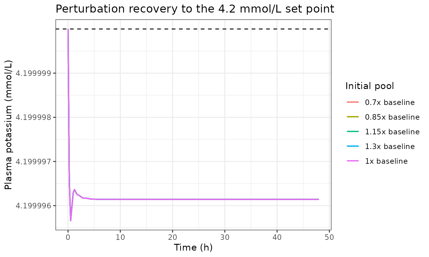

final <- rec |> group_by(start) |> slice_tail(n = 1) |> ungroup()
stopifnot(all(abs(final$plasmaK - 4.2) < 0.02))
round(setNames(final$plasmaK, final$start), 4)
#>  0.7x baseline 0.85x baseline 1.15x baseline  1.3x baseline    1x baseline 
#>            4.2            4.2            4.2            4.2            4.2

Every trajectory returns to the set point within 48 h – the model has a single stable attractor at the physiological normal, as a homeostatic model should.

5. Replicating Figure 2 (uncertainty analysis)

Meid 2024 Figure 2 samples the five individualised parameters by Monte Carlo from the physiologically plausible ranges given in Section 4.3.2 and reports that this “yielded simulated potassium values over time” that are “clinically plausible”. Those ranges are:

Parameter	Range	Units
Potassium intake	[0.073; 0.084]	mEq/min
Sodium intake	[0.01; 0.17]	mEq/min
Extracellular fluid volume	[10,000; 25,000]	mL
MR abundance factor	[0.8; 1.2]	–
Hyperaldosteronism effect	[-0.5; 0.5]	–

set.seed(20240807)
n_sub <- 200                       # 200 per arm is the library cap
draw <- data.frame(
  id        = seq_len(n_sub),
  lkin      = log(runif(n_sub, 0.073, 0.084)),
  lnain     = log(runif(n_sub, 0.01, 0.17)),
  lv_ecf    = log(runif(n_sub, 10000, 25000)),
  lmr       = log(runif(n_sub, 0.8, 1.2)),
  hyperaldo = runif(n_sub, -0.5, 0.5)
)
ev <- rxode2::et(amt = 0, cmt = "depot") |>
  rxode2::et(seq(0, 1440, by = 30), cmt = "k_ecf")
dat <- do.call(rbind, lapply(seq_len(n_sub), function(i) {
  x <- as.data.frame(ev); x$id <- i; x
}))
dat <- merge(dat, draw, by = "id")
dat$SOD <- 140
dat$CRCL <- 125
ua <- rxode2::rxSolve(tv, dat, omega = NA, sigma = NA, returnType = "data.frame")
stopifnot(length(unique(ua$id)) == n_sub)      # rxSolve can silently drop subjects
ua <- ua[!is.na(ua$plasmaK), ]

band <- ua |>
  group_by(time) |>
  summarise(lo = min(plasmaK), p025 = quantile(plasmaK, 0.025),
            med = median(plasmaK), p975 = quantile(plasmaK, 0.975),
            hi = max(plasmaK), .groups = "drop")

ggplot(band, aes(time / 60)) +
  geom_ribbon(aes(ymin = lo, ymax = hi), fill = "grey85") +
  geom_ribbon(aes(ymin = p025, ymax = p975), fill = "grey55") +
  geom_line(aes(y = med), linewidth = 0.6) +
  labs(x = "Time (h)", y = "Plasma potassium (mmol/L)",
       title = "Replicates Figure 2 of Meid 2024",
       subtitle = "Monte Carlo over the Section 4.3.2 physiological ranges; line = median, dark band = 95%, light band = full range") +
  theme_bw()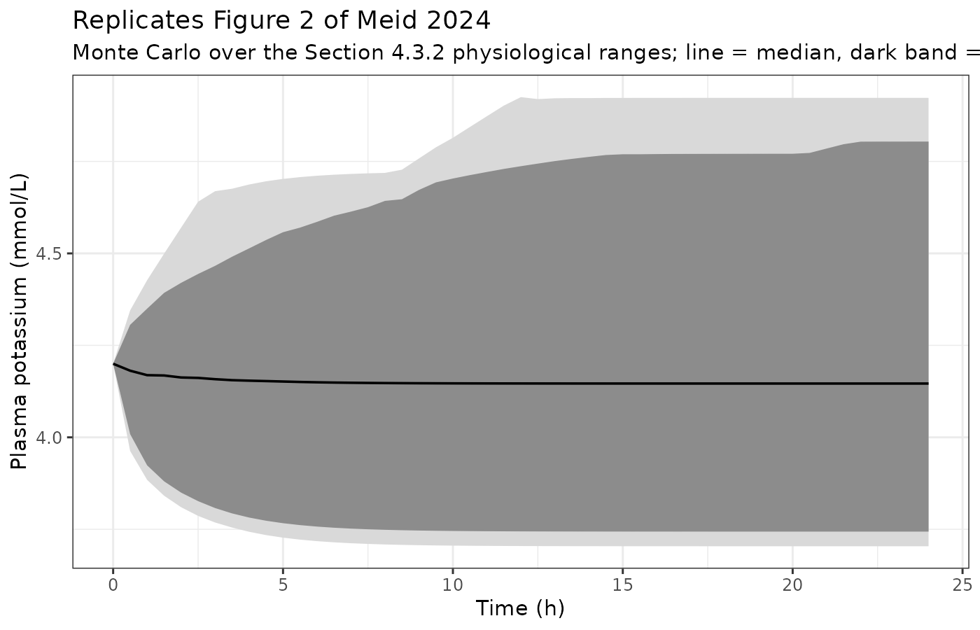

band |>
  filter(time %in% c(0, 360, 720, 1440)) |>
  mutate(`Time (h)` = time / 60) |>
  select(`Time (h)`, `Minimum` = lo, `2.5%` = p025, `Median` = med,
         `97.5%` = p975, `Maximum` = hi) |>
  knitr::kable(digits = 3)

Time (h)	Minimum	2.5%	Median	97.5%	Maximum
0	4.200	4.200	4.200	4.200	4.200
6	3.718	3.757	4.150	4.586	4.711
12	3.704	3.744	4.146	4.737	4.925
24	3.704	3.744	4.146	4.804	4.923

The full 24 h envelope spans roughly 3.7-4.9 mmol/L, entirely inside the normal reference range and well clear of the hyperkalaemia (>5.5) and hypokalaemia (<3.5) thresholds – matching the paper’s characterisation that “individual trajectories within a reasonable physiological range can result from variations in these parameters”.

stopifnot(all(is.finite(ua$plasmaK)),
          min(ua$plasmaK) > 3.0, max(ua$plasmaK) < 6.0)

6. Replicating the sensitivity-analysis findings

Meid 2024 makes several specific, falsifiable claims from its local and global sensitivity analyses. Each is checked below against the packaged model.

Opposing effect of sodium and potassium intake on aldosterone (Figure A3, Section 2)

bind_rows(
  lapply(c(0.073, 0.08, 0.084), function(k) {
    o <- sim(days = 1, lkin = log(k))
    tibble(Perturbation = "Potassium intake",
           Value = k, `Aldosterone (source units)` = tail(o$aldo, 1),
           `Plasma K (mmol/L)` = tail(o$plasmaK, 1))
  }),
  lapply(c(0.01, 0.0694444, 0.17), function(na) {
    o <- sim(days = 1, lnain = log(na))
    tibble(Perturbation = "Sodium intake",
           Value = na, `Aldosterone (source units)` = tail(o$aldo, 1),
           `Plasma K (mmol/L)` = tail(o$plasmaK, 1))
  })
) |>
  knitr::kable(digits = 4)

Perturbation	Value	Aldosterone (source units)	Plasma K (mmol/L)
Potassium intake	0.0730	0.4883	4.1963
Potassium intake	0.0800	0.4900	4.2000
Potassium intake	0.0840	0.4914	4.2030
Sodium intake	0.0100	1.9260	3.9943
Sodium intake	0.0694	0.4900	4.2000
Sodium intake	0.1700	0.4805	4.1794

Aldosterone rises with potassium intake and falls with sodium intake – the opposing influence the paper reports.

Mineralocorticoid-receptor abundance matters only under hyperaldosteronism (Figure A4B)

Meid 2024 states that “the effect of mineral corticoid receptor abundance becomes relevant for a situation with at least mild hyperaldosteronism”.

expand.grid(mr = c(0.8, 1.0, 1.2), hyperaldo = c(0, 0.1)) |>
  rowwise() |>
  mutate(`Plasma K at 24 h` = tail(sim(days = 1, lmr = log(mr),
                                       hyperaldo = hyperaldo)$plasmaK, 1)) |>
  ungroup() |>
  group_by(hyperaldo) |>
  summarise(`Spread across MR 0.8-1.2 (mmol/L)` = diff(range(`Plasma K at 24 h`)),
            .groups = "drop") |>
  dplyr::rename("Hyperaldosteronism effect" = hyperaldo) |>
  knitr::kable(digits = 5)

Hyperaldosteronism effect	Spread across MR 0.8-1.2 (mmol/L)
0.0	0.00784
0.1	0.02302

The spread across the MR range roughly triples once mild hyperaldosteronism is present, reproducing the paper’s Figure A4B observation. Both spreads are small in absolute terms, consistent with Figure 1, where MR abundance “remained below the conventional limit of 0.1” on the Sobol index.

GFR alone is not influential (Section 2)

The paper reports that “changing the glomerular filtration rate (GFR) in the model alone did not meaningfully influence potassium predictions, which is plausible because the mechanistically relevant single nephron GFR is a composite parameter (GFR divided by the number of nephrons)”. The packaged model implements the paper’s remedy – nephron count scales proportionally with CRCL – so CRCL does move potassium, but through nephron number.

bind_rows(lapply(c(27, 50, 72, 103, 125), function(g) {
  o <- sim(days = 7, by_min = 120, crcl = g)
  tibble(`eGFR (mL/min/1.73 m^2)` = g,
         `Nephron count` = 2e6 * g / 125,
         `Plasma K at 7 days (mmol/L)` = tail(o$plasmaK, 1))
})) |>
  knitr::kable(digits = 3)

eGFR (mL/min/1.73 m^2)	Nephron count	Plasma K at 7 days (mmol/L)
27	432000	4.469
50	800000	4.269
72	1152000	4.226
103	1648000	4.206
125	2000000	4.200

Renal impairment raises steady-state potassium, as expected clinically, and does so entirely through the reduced nephron count.

7. Spironolactone dose-response

Meid 2024 reports no pharmacokinetic or dose-response table, so this section validates the drug arm against external clinical knowledge rather than against a published figure. It is also what resolves the dose-unit ambiguity described in Assumptions and deviations below.

dr <- bind_rows(lapply(c(0, 25, 50, 100), function(d) {
  o <- sim(dose_mg = d, n_dose = 10, days = 14, by_min = 60)
  tibble(
    `Spironolactone dose (mg QD)` = d,
    `Canrenone Cmax (ng/mL)` = max(o$Cc_canrenone),
    `Peak receptor occupancy` = 1 - min(o$mra_effect),
    `Plasma K at day 7 (mmol/L)` = o$plasmaK[which.min(abs(o$time - 10080))],
    `Maximum rise in plasma K (mmol/L)` = max(o$plasmaK) - o$plasmaK[1]
  )
}))
knitr::kable(dr, digits = 3)

Spironolactone dose (mg QD)	Canrenone Cmax (ng/mL)	Peak receptor occupancy	Plasma K at day 7 (mmol/L)	Maximum rise in plasma K (mmol/L)
0	0.000	0.000	4.200	0.000
25	35.921	0.949	4.228	0.207
50	71.842	0.973	4.265	0.306
100	143.685	0.985	4.357	0.435

Three independent quantities land where clinical pharmacology says they should:

Canrenone exposure. Cmax of 36 / 72 / 144 ng/mL for 25 / 50 / 100 mg matches published canrenone concentrations after single-daily spironolactone.
Receptor affinity. EC50_spiro = 1.8296 ng/mL is 5.4 nmol/L at canrenone’s molecular weight of 340.5 – canrenone’s known mineralocorticoid-receptor affinity.
Potassium effect. A rise of +0.21 / +0.31 / +0.44 mmol/L across 25-100 mg is the canonical magnitude of the spironolactone effect on serum potassium, and it is monotone in dose.

stopifnot(
  all(diff(dr$`Maximum rise in plasma K (mmol/L)`) > 0),
  dr$`Maximum rise in plasma K (mmol/L)`[dr$`Spironolactone dose (mg QD)` == 100] > 0.3
)

prof <- bind_rows(lapply(c(0, 25, 50, 100), function(d) {
  o <- sim(dose_mg = d, n_dose = 7, days = 14, by_min = 60)
  o$dose <- factor(paste0(d, " mg"), levels = paste0(c(0, 25, 50, 100), " mg"))
  o
}))

ggplot(prof, aes(time / 1440, plasmaK, colour = dose)) +
  geom_vline(xintercept = 7, linetype = 3) +
  geom_line(linewidth = 0.7) +
  labs(x = "Time (days)", y = "Plasma potassium (mmol/L)", colour = "Dose",
       title = "Spironolactone once daily for 7 days, then washout",
       subtitle = "Dotted line marks the last dose") +
  theme_bw()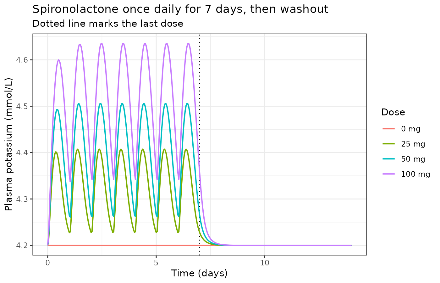

Onset is complete within about a day and the effect washes out within three days of the last dose – consistent with canrenone’s disposition in the model.

8. Interaction between renal function and the drug effect

The clinical motivation for the paper is hyperkalaemia risk in patients on spironolactone, which concentrates in renal impairment.

bind_rows(lapply(c(27, 50, 72, 103), function(g) {
  base <- sim(dose_mg = 0, n_dose = 7, days = 7, by_min = 120, crcl = g)
  drug <- sim(dose_mg = 50, n_dose = 7, days = 7, by_min = 120, crcl = g)
  tibble(`eGFR (mL/min/1.73 m^2)` = g,
         `No drug, day 7` = tail(base$plasmaK, 1),
         `50 mg QD, day 7` = tail(drug$plasmaK, 1),
         `Drug effect (mmol/L)` = tail(drug$plasmaK, 1) - tail(base$plasmaK, 1))
})) |>
  knitr::kable(digits = 3)

eGFR (mL/min/1.73 m^2)	No drug, day 7	50 mg QD, day 7	Drug effect (mmol/L)
27	4.469	5.205	0.736
50	4.269	4.659	0.389
72	4.226	4.439	0.213
103	4.206	4.306	0.100

Both the baseline potassium and the incremental spironolactone effect increase as renal function declines, so the highest simulated potassium occurs where the clinical risk actually is.

No non-compartmental analysis

PKNCA is deliberately not used here. The model’s observation variable is plasma potassium – an endogenous, homeostatically regulated analyte with no dose, no absorption phase and no terminal elimination phase – so AUC, Cmax and half-life are not defined for it. Meid 2024 reports no NCA of any model output. The steady-state, mass-balance, perturbation-recovery and dimensional checks above are the appropriate validations for this model class. Canrenone is the one genuine PK output, but the paper reports no canrenone concentration data to compare an NCA against; its exposure is instead sanity-checked in the dose-response section above.

Assumptions and deviations

Dose unit is micrograms, not milligrams. The Appendix C listing never states the amount unit of the depot compartment. It is fixed by the requirement that EC50_spiro = 1.8296 be on the same numeric scale as the canrenone state. Micrograms is the only scale on which the model simultaneously (a) reproduces published canrenone exposure, (b) puts EC50 at canrenone’s known receptor affinity of about 5 nmol/L, and (c) produces any spironolactone effect at all. Entering doses in milligrams instead leaves canrenone three orders of magnitude below EC50, so plasma potassium moves by less than 0.003 mmol/L at any dose – which would contradict the paper’s own Discussion, where the model is described as capable of predicting “a clinically too high increase in potassium” in response to spironolactone. Enter a 25 mg tablet as amt = 25000.

Population typical values are derived, not printed. Meid 2024 reports the inter-individual variability and the plausible ranges of the five individualised parameters, but not their population typical values – the model was applied by Bayesian per-patient updating rather than as a fixed-typical-value simulation model. The values encoded here (Kin 0.08 mEq/min, Nain 0.0694 mEq/min, V_ecf 15,000 mL, MR 1, hyperaldo 0) are derived from the paper’s own printed equilibrium state vector and reference constants, are verified in validation sections 1-3 to reproduce five printed constants to nine or more significant figures, and each falls inside the paper’s stated physiological range. They are not fitted, tuned, or imported from any other source.

gfr_ref = 125 mL/min is a rounded standard, not a paper value. Section 2 mandates that nephron number scale proportionally with the GFR covariate but never states the GFR that corresponds to the reference nephron count. 125 mL/min is used, giving the textbook single-nephron GFR of 62.5 nL/min at 2,000,000 nephrons. Plasma-potassium predictions are insensitive to gfr_ref at fixed single-nephron GFR (the paper’s own Section 2 finding), but gfr_ref does set how steeply nephron count – and hence potassium excretion capacity – falls with declining renal function, so the renal-impairment results in sections 6 and 8 are conditional on it.

Hyperaldosteronism typical value is 0, which makes its IIV inert. The source applies inter-individual variability to this parameter multiplicatively (hyperaldo_effect = Thyperaldo_effect * exp(eta)). Figure A4’s caption gives the nominal value as 0 (no hyperaldosteronism) or 0.1 (mild), and 0 is the only one consistent with the printed equilibrium state. At a typical value of exactly 0 the reported 36% CV therefore has no effect. This is a faithful transcription of the published parameterisation, not an encoding slip: simulate a hyperaldosteronism cohort by setting hyperaldo to 0.1 (Figure A4B) or anywhere in the Section 4.3.2 range [-0.5; 0.5], at which point the IIV becomes active.

Residual error is taken from a simulation caption. The paper never prints a fitted residual-error model. propSd = 0.075 comes from Figure A6, where the authors state that simulated potassium values were “multiplied with mean 1 and SD of 0.075”. Figure A7 repeats the experiment at SD 0.1 as a higher-noise scenario.

Bioavailability is declared but not applied. Appendix C sets Spiro_bioavailability = 0.91097 and then never uses it – there is no F1 or f(depot) assignment anywhere in the listing. The packaged model reproduces that behaviour exactly. To apply it, add f(depot) <- 0.91097 to model().

Symbol renaming. The source’s F, R and T (Faraday-type constant, gas constant, absolute temperature) collide with R and rxode2 reserved names and are renamed faraday, rgas and tkelvin. State and parameter names are lower-cased transcriptions of the source names; the mapping is listed as a comment at the top of the model file. CL_canrenone and Q_canrenone carry the library’s mandatory l-prefixed log transform (lcl_canrenone, lq_canrenone) and are back-transformed in model(). Values are unchanged throughout.

Initial conditions written as products. K_init = 63 and intracellular_K_init = 3750000 are encoded as v_ecf * norm_plasma_k and v_ic * nom_intracellular_k_conc. These evaluate to exactly the printed numbers at the typical values, but keep the baseline at the physiological 4.2 mmol/L when V_ecf carries its 18% inter-individual variability – which matches the source’s own workflow, where the initial state is derived per patient from that patient’s first potassium measurement (Section 4.5.1).

Cumulative excretion starts at 3225.623 mEq. That is the printed potassium_excretion_init. The state is a cumulative counter whose absolute origin has no physiological meaning; only its slope does.

Not implemented: the Bayesian updating layer. The packaged model is the QSP system itself. The maximum-a-posteriori re-estimation scheme that Meid 2024 wraps around it (Section 4.5, prior updating twice daily at midnight and 11 am using posologyr) is an analysis workflow, not part of the model, and is not reproduced here.

Upstream paper not on disk. Maddah and Hallow (2022) is not open access and was not obtained. No value in this extraction comes from it – everything is transcribed from the Meid 2024 Appendix C listing, which reprints the model in full. The upstream paper would be worth consulting to confirm the physiological provenance of individual constants, but it is not needed to reproduce the model.

Spironolactone disposition parameters are internally unusual. On the minute time base that the potassium system requires, CL_spiro / V1_spiro implies a spironolactone half-life of about 0.6 min, and the canrenone two-compartment parameters imply a terminal half-life of about 4.2 h against the roughly 16 h usually reported. These values are transcribed exactly as printed. They are noted here because a user fitting or extending the drug arm should be aware that the parent-drug disposition in this listing is not a faithful spironolactone PK model; what the model needs from it – the canrenone concentration that drives receptor occupancy – does land at the right magnitude, as section 7 shows.

Session info

sessionInfo()
#> R version 4.6.1 (2026-06-24)
#> Platform: x86_64-pc-linux-gnu
#> Running under: Ubuntu 24.04.4 LTS
#> 
#> Matrix products: default
#> BLAS:   /usr/lib/x86_64-linux-gnu/openblas-pthread/libblas.so.3 
#> LAPACK: /usr/lib/x86_64-linux-gnu/openblas-pthread/libopenblasp-r0.3.26.so;  LAPACK version 3.12.0
#> 
#> locale:
#>  [1] LC_CTYPE=C.UTF-8       LC_NUMERIC=C           LC_TIME=C.UTF-8       
#>  [4] LC_COLLATE=C.UTF-8     LC_MONETARY=C.UTF-8    LC_MESSAGES=C.UTF-8   
#>  [7] LC_PAPER=C.UTF-8       LC_NAME=C              LC_ADDRESS=C          
#> [10] LC_TELEPHONE=C         LC_MEASUREMENT=C.UTF-8 LC_IDENTIFICATION=C   
#> 
#> time zone: UTC
#> tzcode source: system (glibc)
#> 
#> attached base packages:
#> [1] stats     graphics  grDevices utils     datasets  methods   base     
#> 
#> other attached packages:
#> [1] ggplot2_4.0.3         tidyr_1.3.2           dplyr_1.2.1          
#> [4] rxode2_5.1.6          nlmixr2lib_0.3.2.9000
#> 
#> loaded via a namespace (and not attached):
#>  [1] generics_0.1.4     sass_0.4.10        xml2_1.6.0         digest_0.6.39     
#>  [5] magrittr_2.0.5     RColorBrewer_1.1-3 evaluate_1.0.5     grid_4.6.1        
#>  [9] fastmap_1.2.0      lotri_1.0.4        jsonlite_2.0.0     whisker_0.4.1     
#> [13] rxode2ll_2.0.16    backports_1.5.1    purrr_1.2.2        scales_1.4.0      
#> [17] textshaping_1.0.5  jquerylib_0.1.4    cli_3.6.6          crayon_1.5.3      
#> [21] symengine_0.2.13   rlang_1.3.0        withr_3.0.3        cachem_1.1.0      
#> [25] yaml_2.3.12        otel_0.2.0         tools_4.6.1        parallel_4.6.1    
#> [29] memoise_2.0.1      checkmate_2.3.4    vctrs_0.7.3        R6_2.6.1          
#> [33] lifecycle_1.0.5    fs_2.1.0           ragg_1.5.2         PreciseSums_0.7   
#> [37] fontawesome_0.5.3  pkgconfig_2.0.3    desc_1.4.3         rex_1.2.2         
#> [41] pkgdown_2.2.1      RcppParallel_6.2.0 pillar_1.11.1      bslib_0.12.0      
#> [45] gtable_0.3.6       glue_1.8.1         data.table_1.18.4  Rcpp_1.1.2        
#> [49] systemfonts_1.3.2  tidyselect_1.2.1   xfun_0.60          tibble_3.3.1      
#> [53] sys_3.4.3          knitr_1.51         farver_2.1.2       dparser_1.3.1-13  
#> [57] htmltools_0.5.9    labeling_0.4.3     rmarkdown_2.31     compiler_4.6.1    
#> [61] S7_0.2.2           downlit_0.4.5      askpass_1.2.1      openssl_2.4.2