Abrocitinib (Wojciechowski 2022)
Source:vignettes/articles/Wojciechowski_2022_abrocitinib.Rmd
Wojciechowski_2022_abrocitinib.RmdModel and source
- Citation: Wojciechowski J, Malhotra BK, Wang X, Fostvedt L, Valdez H, Nicholas T. Population Pharmacokinetics of Abrocitinib in Healthy Individuals and Patients with Psoriasis or Atopic Dermatitis. Clin Pharmacokinet. 2022;61:709-723. doi:10.1007/s40262-021-01104-z. Model equations from the Online Resource 2 NONMEM control stream.
- Description: Two-compartment population PK model for oral abrocitinib (JAK1 inhibitor) in healthy adults and in adolescents and adults with psoriasis or atopic dermatitis (Wojciechowski 2022). Parallel first-order (depot) and zero-order (central) absorption, with the first-order arm capped at a fixed amount per dose; an absorption lag for tablets; absolute oral bioavailability on the logit scale anchored at 0.5977 with additive shifts for formulation, repeated dosing, CYP DDIs, race, disease, hepatic impairment, adolescence, sex and the 800 mg dose; clearance that falls exponentially with time on treatment and depends on the effective (bioavailable) daily dose; allometric weight scaling; and a study-specific proportional residual error.
- Article: https://doi.org/10.1007/s40262-021-01104-z (open access, Clin Pharmacokinet 2022;61:709-723)
- Supplement: Online Resource 1-4 at the same DOI; Online Resource 2 prints the final NONMEM control stream from which every model equation below is taken.
A correction notice (Clin Pharmacokinet, published online 18 February 2022) changed only the article’s licence to open access; no value was revised.
Population
The model was fitted to 6206 abrocitinib plasma concentrations from 995 participants in 11 Pfizer studies run between May 2013 and July 2019: seven phase I studies in healthy volunteers (including dedicated food, formulation, drug-interaction, hepatic-impairment and QT studies), one phase II study in plaque psoriasis, and one phase IIb and two phase III studies in moderate-to-severe atopic dermatitis (Online Resource 1). By participant type there were 165 healthy volunteers, 45 patients with psoriasis, 769 with atopic dermatitis (90 of them adolescents aged 12-17 years) and 8 each with mild and moderate hepatic impairment (Child-Pugh A and B). Overall 39.2% were female; median age was 34 years (range 12-84) and median body weight 76 kg (range 34.4-180); 66.6% were White, 11.0% Black, 17.9% Asian (4.4% Japanese) and 4.0% other race (Table 1). Daily doses ranged from 3 to 800 mg.
The same information is available programmatically:
str(readModelDb("Wojciechowski_2022_abrocitinib")()$population)
#> List of 14
#>  $ species       : chr "human"
#>  $ n_subjects    : int 995
#>  $ n_studies     : int 11
#>  $ n_observations: int 6206
#>  $ age_range     : chr "12-84 years"
#>  $ age_median    : chr "34 years"
#>  $ weight_range  : chr "34.4-180 kg"
#>  $ weight_median : chr "76 kg"
#>  $ sex_female_pct: num 39.2
#>  $ race_ethnicity: Named num [1:5] 66.6 11 17.9 4 0.5
#>   ..- attr(*, "names")= chr [1:5] "White" "Black" "Asian" "Other" ...
#>  $ disease_state : chr "Healthy volunteers (n = 165), moderate-to-severe plaque psoriasis (n = 45), moderate-to-severe atopic dermatiti"| __truncated__
#>  $ dose_range    : chr "3-800 mg/day oral (single doses 3-800 mg; 10-400 mg once daily or 100-200 mg twice daily)"
#>  $ regions       : chr "Multinational (Western and Japanese participants)"
#>  $ notes         : chr "Seven phase I, two phase II and two phase III studies (Online Resource 1). Demographics from Table 1. Most conc"| __truncated__
Source trace
Every value is in Table 2 of the paper; every equation is in the
Online Resource 2 control stream. The per-parameter origin is also
recorded next to each ini() entry in
inst/modeldb/specificDrugs/Wojciechowski_2022_abrocitinib.R.
| Equation / parameter | Value | Source location |
|---|---|---|
lcl |
log(22) L/h | Table 2 ‘CL’ |
lvc |
log(87.8) L | Table 2 ‘Vc’ |
lq |
log(1.16) L/h | Table 2 ‘Q’ |
lvp |
log(8.25) L | Table 2 ‘Vp’ |
lr1 |
log(75.3) mg/h | Table 2 ‘k0’ (zero-order rate into central) |
lamt_fo |
log(121) mg | Table 2 ‘AK1’ (amount absorbed first-order) |
lka |
log(4.01) 1/h | Table 2 ‘ka’ |
ltlag |
log(0.183) h | Table 2 ‘Effect of tablet formulations on ALAG1’; base ALAG1 = 0 (Online Resource 2) |
logitfdepot |
logit(0.5977), held constant | Methods 2.4.2; Online Resource 2 POPF = 0.5977
|
e_rif_f, e_cypinh_f
|
-2.08, 1.31 | Table 2 rifampin / fluconazole-or-fluvoxamine on F |
e_ph2b_f, e_ph3_f
|
-1.02, -0.766 | Table 2 phase IIb / phase III tablet on F |
e_multidose_f |
0.241 | Table 2 ‘Effect of multiple dosing on F’ |
e_race_f, e_dis_f,
e_hepimp_f
|
0.815, 0.489, 1.3 | Table 2 Asian/other race, psoriasis and AD, hepatic impairment on F |
e_adol_f, e_dose800_f,
e_sexf_f
|
-0.589, -0.778, 0.353 | Table 2 adolescent age, 800 mg dose, female sex on F |
e_highfat_amt_fo |
-1, held constant | Table 2 ‘Effect of high-fat meal on Ak1’; Online Resource 3 run 133 |
e_susp_amt_fo, e_ph2b_amt_fo
|
1.17, -0.68 | Table 2 suspension / phase IIb tablets on Ak1 |
e_rif_cl, e_fluco_cl,
e_fluvox_cl
|
0.264, -0.541, -0.234 | Table 2 DDI effects on CL |
e_dose_cl |
-0.169 | Table 2 ‘Effect of effective daily dose on CL’ |
cl_exp_famp |
-0.186 | Table 2 ‘Maximum change in CL with respect to time (TAFO)’ |
lcl_exp_kdes |
log(log(2) / 21.6) 1/h | Table 2 half-life 21.6 h |
e_wt_cl, e_wt_vc
|
0.453, 0.52 | Table 2 weight on CL and Q / Vc and Vp |
etalcl, etalvc
|
0.577^2, 0.414^2, cov 0.326 x 0.577 x 0.414 | Table 2 IIV (CV = sqrt(omega^2), footnote a) and correlation |
propSd, addSd
|
0.437, 0.509 ng/mL | Table 2 RUV PRO / RUV ADD (SDs; EPS variance 1) |
e_studymod_propSd, e_studyhi_propSd
|
0.495, 1.16 | Table 2 study effects on RUV PRO; studies from Online Resource 2 |
logit_fi / fi
|
sum of logit shifts, expit()
|
Online Resource 2 FT, FI
|
ffo = min(1, amt_fo / DOSE) |
n/a | Online Resource 2 POPFK1
|
cl |
weight, DDI, time and effective-dose terms | Online Resource 2 CL, COVTAFOCL,
COVEFFDOSRCL
|
f(depot), f(central),
rate(central)
|
fi * ffo, fi * (1 - ffo),
r1
|
Online Resource 2 F1, F2,
R2
|
alag(depot), alag(central)
|
tablet lag | Online Resource 2 ALAG1,
ALAG2 = ALAG1
|
Cc ~ add(addSd) + prop(propSd_study) |
n/a | Online Resource 2 $ERROR
(W = SQRT(IPRE^2 * RUVPRO^2 + RUVADD^2)) |
Dosing the model
The paper’s dataset gives every administration two records with the
same amount: one into the depot (first-order arm) and one into the
central compartment with RATE = -1, so that the model
supplies the zero-order rate. The same is required here: a
depot record with rate = 0 and a
central record with rate = -1. The model then
routes fi * ffo of the dose to the depot and
fi * (1 - ffo) to central at 75.3 mg/h, where
ffo is min(1, 121 mg / dose) for tablets. A
100 mg tablet dose is therefore absorbed entirely first-order, and the
zero-order arm only appears above 121 mg (or always, after a high-fat
meal).
Covariates are columns of the event table.
DOSE_ABROCITINIB_MG must equal amt;
DOSE_ABROCITINIB_MGD is the regimen’s total daily dose;
MULTI_DOSE is 0 up to the second dose of a regimen and 1
from then on. Time-dependent clearance runs on the solver time
t, so the first dose of a treatment period must sit at
t = 0.
reference_covariates <- function(...) {
  base <- list(
    WT = 70, SEXF = 0, RACE_ASIAN = 0, RACE_OTHER = 0, ADOLESCENT = 0,
    DIS_PSORIASIS = 0, DIS_ATOPIC_DERMATITIS = 0,
    HEPIMP_MILD = 0, HEPIMP_MOD = 0,
    CONMED_RIFAMPICIN = 0, CONMED_FLUCONAZOLE = 0, CONMED_FLUVOXAMINE = 0,
    FED_HIGHFAT = 0,
    FORM_ABROCITINIB_SUSP = 0, FORM_ABROCITINIB_TAB_PH2B = 0,
    FORM_ABROCITINIB_TAB_PH3 = 1,
    DOSE_ABROCITINIB_MG = 200, DOSE_ABROCITINIB_MGD = 200,
    STUDY_B7451005 = 0, STUDY_B7451006 = 0, STUDY_B7451012 = 0,
    STUDY_B7451043 = 0
  )
  as.data.frame(utils::modifyList(base, list(...)))
}

# One subject's event table: n_dose administrations every `tau` hours, each
# as a depot record and a rate = -1 central record, plus observations on the
# central state. Covariates in `cov` (one row) are copied to every row;
# MULTI_DOSE switches to 1 at the second dose.
regimen_events <- function(id, cov, n_dose, tau = 24, obs_times) {
  dose_times <- (seq_len(n_dose) - 1) * tau
  amt <- cov$DOSE_ABROCITINIB_MG
  doses <- dplyr::bind_rows(
    data.frame(time = dose_times, amt = amt, evid = 1L, cmt = "depot", rate = 0),
    data.frame(time = dose_times, amt = amt, evid = 1L, cmt = "central", rate = -1)
  )
  obs <- data.frame(time = obs_times, amt = 0, evid = 0L, cmt = "central", rate = 0)
  ev <- dplyr::bind_rows(doses, obs) |>
    dplyr::arrange(time, dplyr::desc(evid)) |>
    dplyr::mutate(id = id)
  ev <- cbind(ev, cov[rep(1, nrow(ev)), , drop = FALSE])
  ev$MULTI_DOSE <- as.integer(n_dose > 1 & ev$time >= tau)
  ev
}
Reproducing the published covariate ratios
Figure 3 of the paper gives, for each covariate scenario, the median over 1000 simulated trials of the geometric-mean ratio of steady-state Cmax and 24-h AUC after 200 mg once daily, relative to a healthy, White, adult, male, 70 kg, fasted participant taking the phase III tablet. The Results text adds three typical-patient comparisons. All are reproduced below with the typical-value model (random effects set to zero) after 30 days of dosing; PKNCA computes Cmax and AUC over the last dosing interval.
mod <- readModelDb("Wojciechowski_2022_abrocitinib")
mod_typical <- rxode2::zeroRe(mod)
#> ℹ parameter labels from comments will be replaced by 'label()'

scenarios <- list(
  "Reference" = reference_covariates(),
  "Female" = reference_covariates(SEXF = 1),
  "Adolescent" = reference_covariates(ADOLESCENT = 1),
  "Asian/other" = reference_covariates(RACE_ASIAN = 1),
  "Rifampin DDI" = reference_covariates(CONMED_RIFAMPICIN = 1),
  "Fluconazole DDI" = reference_covariates(CONMED_FLUCONAZOLE = 1),
  "Fluvoxamine DDI" = reference_covariates(CONMED_FLUVOXAMINE = 1),
  "AD/psoriasis patient" = reference_covariates(DIS_ATOPIC_DERMATITIS = 1),
  "Mild/moderate hepatic impairment" = reference_covariates(HEPIMP_MILD = 1),
  "High body weight (111 kg)" = reference_covariates(WT = 111),
  "Low body weight (52 kg)" = reference_covariates(WT = 52),
  "Phase II tablet 400 mg, fasted" = reference_covariates(
    FORM_ABROCITINIB_TAB_PH3 = 0, DOSE_ABROCITINIB_MG = 400,
    DOSE_ABROCITINIB_MGD = 400
  ),
  "Phase II tablet 400 mg, high-fat meal" = reference_covariates(
    FORM_ABROCITINIB_TAB_PH3 = 0, DOSE_ABROCITINIB_MG = 400,
    DOSE_ABROCITINIB_MGD = 400, FED_HIGHFAT = 1
  ),
  "AD, White, 80 kg" = reference_covariates(WT = 80, DIS_ATOPIC_DERMATITIS = 1),
  "AD, Asian, 66 kg" = reference_covariates(
    WT = 66, DIS_ATOPIC_DERMATITIS = 1, RACE_ASIAN = 1
  ),
  "AD, adolescent, 61 kg" = reference_covariates(
    WT = 61, DIS_ATOPIC_DERMATITIS = 1, ADOLESCENT = 1
  )
)

n_days <- 30
last_day <- seq((n_days - 1) * 24, n_days * 24, by = 0.05)
ev_typ <- dplyr::bind_rows(lapply(seq_along(scenarios), function(i) {
  regimen_events(i, scenarios[[i]], n_dose = n_days, obs_times = last_day) |>
    dplyr::mutate(scenario = names(scenarios)[i])
}))

sim_typ <- rxode2::rxSolve(
  mod_typical, ev_typ, keep = "scenario", returnType = "data.frame"
)
#> ℹ omega/sigma items treated as zero: 'etalcl', 'etalvc'
#> Warning: multi-subject simulation without without 'omega'

conc_typ <- sim_typ |>
  dplyr::filter(!is.na(Cc)) |>
  dplyr::select(id, scenario, time, Cc)
dose_typ <- ev_typ |>
  dplyr::filter(evid == 1, cmt == "depot") |>
  dplyr::select(id, scenario, time, amt)

nca_typ <- PKNCA::pk.nca(PKNCA::PKNCAdata(
  PKNCA::PKNCAconc(conc_typ, Cc ~ time | scenario + id),
  PKNCA::PKNCAdose(dose_typ, amt ~ time | scenario + id),
  intervals = data.frame(
    start = (n_days - 1) * 24, end = n_days * 24, cmax = TRUE, auclast = TRUE
  )
))

typ <- as.data.frame(nca_typ) |>
  dplyr::filter(PPTESTCD %in% c("cmax", "auclast")) |>
  dplyr::select(scenario, PPTESTCD, PPORRES) |>
  tidyr::pivot_wider(names_from = PPTESTCD, values_from = PPORRES)
ref <- typ[typ$scenario == "Reference", ]
published <- tibble::tribble(
  ~scenario, ~versus, ~pub_cmax, ~pub_auc, ~source,
  "Female", "Reference", 0.996, 0.999, "Figure 3",
  "Adolescent", "Reference", 0.686, 0.666, "Figure 3",
  "Asian/other", "Reference", 1.430, 1.510, "Figure 3",
  "Rifampin DDI", "Reference", 0.186, 0.128, "Figure 3",
  "Fluconazole DDI", "Reference", 2.010, 3.840, "Figure 3",
  "Fluvoxamine DDI", "Reference", 1.730, 2.320, "Figure 3",
  "AD/psoriasis patient", "Reference", 1.270, 1.310, "Figure 3",
  "Mild/moderate hepatic impairment", "Reference", 1.650, 1.780, "Figure 3 and Discussion",
  "High body weight (111 kg)", "Reference", 0.789, 0.800, "Figure 3",
  "Low body weight (52 kg)", "Reference", 1.170, 1.150, "Figure 3",
  "Phase II tablet 400 mg, high-fat meal", "Phase II tablet 400 mg, fasted", 1.010, 0.991, "Figure 3",
  "AD, Asian, 66 kg", "AD, White, 80 kg", 1.43, 1.48, "Results 3.4",
  "AD, adolescent, 61 kg", "AD, White, 80 kg", 0.86, 0.81, "Discussion (14% and 19% lower)"
)

ratios <- published |>
  dplyr::left_join(typ, by = "scenario") |>
  dplyr::left_join(
    dplyr::rename(typ, versus = scenario, cmax_ref = cmax, auc_ref = auclast),
    by = "versus"
  ) |>
  dplyr::mutate(
    sim_cmax = cmax / cmax_ref,
    sim_auc = auclast / auc_ref,
    diff_cmax_pct = 100 * (sim_cmax / pub_cmax - 1),
    diff_auc_pct = 100 * (sim_auc / pub_auc - 1)
  )

ratios |>
  dplyr::transmute(
    "Scenario" = scenario,
    "Compared with" = versus,
    "Cmax ratio, model" = signif(sim_cmax, 3),
    "Cmax ratio, paper" = pub_cmax,
    "AUC ratio, model" = signif(sim_auc, 3),
    "AUC ratio, paper" = pub_auc,
    "Paper source" = source
  ) |>
knitr::kable(caption = "Steady-state ratios after 200 mg once daily (400 mg for the food rows): typical-value model vs. the paper.")| Scenario | Compared with | Cmax ratio, model | Cmax ratio, paper | AUC ratio, model | AUC ratio, paper | Paper source |
|---|---|---|---|---|---|---|
| Female | Reference | 1.200 | 0.996 | 1.220 | 0.999 | Figure 3 |
| Adolescent | Reference | 0.690 | 0.686 | 0.660 | 0.666 | Figure 3 |
| Asian/other | Reference | 1.440 | 1.430 | 1.510 | 1.510 | Figure 3 |
| Rifampin DDI | Reference | 0.193 | 0.186 | 0.129 | 0.128 | Figure 3 |
| Fluconazole DDI | Reference | 1.950 | 2.010 | 3.870 | 3.840 | Figure 3 |
| Fluvoxamine DDI | Reference | 1.730 | 1.730 | 2.320 | 2.320 | Figure 3 |
| AD/psoriasis patient | Reference | 1.270 | 1.270 | 1.310 | 1.310 | Figure 3 |
| Mild/moderate hepatic impairment | Reference | 1.650 | 1.650 | 1.770 | 1.780 | Figure 3 and Discussion |
| High body weight (111 kg) | Reference | 0.790 | 0.789 | 0.812 | 0.800 | Figure 3 |
| Low body weight (52 kg) | Reference | 1.160 | 1.170 | 1.140 | 1.150 | Figure 3 |
| Phase II tablet 400 mg, high-fat meal | Phase II tablet 400 mg, fasted | 0.962 | 1.010 | 1.000 | 0.991 | Figure 3 |
| AD, Asian, 66 kg | AD, White, 80 kg | 1.430 | 1.430 | 1.480 | 1.480 | Results 3.4 |
| AD, adolescent, 61 kg | AD, White, 80 kg | 0.853 | 0.860 | 0.810 | 0.810 | Discussion (14% and 19% lower) |
# Deterministic on the model side; the paper's values are medians of 1000
# simulated trials, so a few percent separates the two.
gated <- dplyr::filter(ratios, scenario != "Female")
stopifnot(
  all(abs(gated$diff_auc_pct) < 3),
  all(abs(gated$diff_cmax_pct) < 6)
)
Apart from the female row, discussed below, every AUC ratio is reproduced to within 1.4% and every Cmax ratio to within 4.7%. That is the agreement expected between a typical-value calculation and the median of the paper’s simulated trials, which include random effects on CL and Vc.
Female sex. Table 2 and the control stream estimate
a +0.353 shift on logit F for females
(IF (SEX.EQ.2) COVSEXF = SEXF2), which the model
reproduces. At the reference this raises steady-state AUC by about 22%,
yet the Female row of Figure 3 is centred at 1.0 (0.996 for Cmax, 0.999
for AUC). The paper does not discuss sex in its Results, so the figure
cannot be reconciled with the estimate it prints. The model keeps the
published estimate, and the row is excluded from the gate above.
ratios |>
  dplyr::filter(versus == "Reference") |>
  dplyr::select(scenario, sim_cmax, pub_cmax, sim_auc, pub_auc) |>
  tidyr::pivot_longer(-scenario, names_to = c("source", "metric"), names_sep = "_") |>
  dplyr::mutate(
    source = dplyr::recode(source, sim = "Model (typical value)", pub = "Paper (Figure 3 median)"),
    metric = dplyr::recode(metric, cmax = "Steady-state Cmax", auc = "24-h AUC")
  ) |>
  ggplot(aes(value, scenario, shape = source, colour = source)) +
  annotate("rect", xmin = 0.8, xmax = 1.25, ymin = -Inf, ymax = Inf, alpha = 0.15, fill = "steelblue") +
  geom_vline(xintercept = 1, linetype = 2) +
  geom_point(size = 2) +
  scale_x_log10() +
  facet_wrap(~metric) +
  labs(x = "Ratio to the reference participant (log scale)", y = NULL, shape = NULL, colour = NULL) +
  theme_bw() +
  theme(legend.position = "bottom")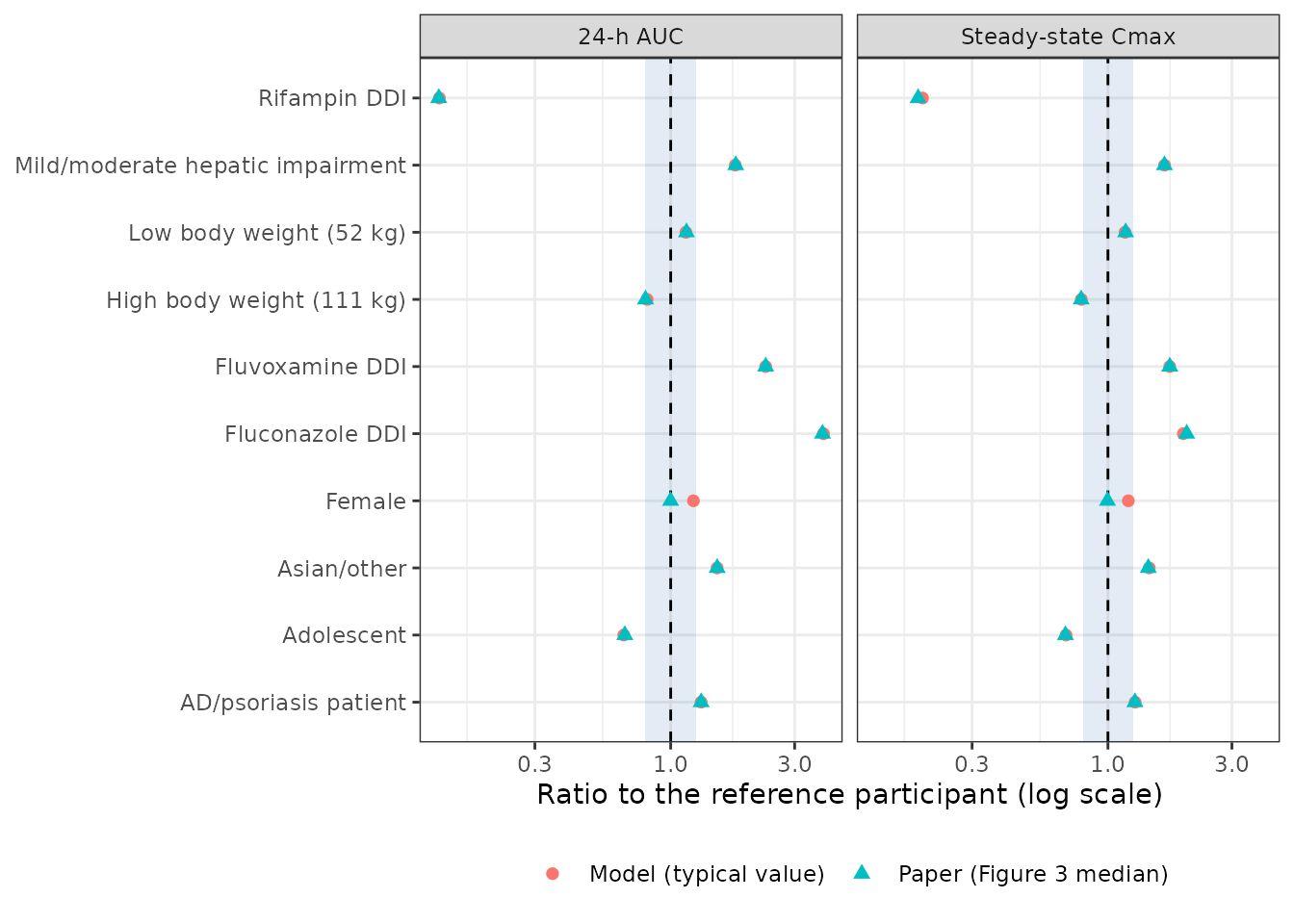
Replicates Figure 3 of Wojciechowski 2022 (median ratios only).
Stochastic simulation in atopic dermatitis
A virtual cohort of atopic-dermatitis patients receives the phase III tablet once daily for 28 days at 100 mg or 200 mg (200 per arm). Covariates follow the atopic-dermatitis column of Table 1: 45.5% female, 21.1% Asian and 2.6% other race, 11.7% adolescents, body weight log-normal around the 73.9 kg median (truncated to the observed 34.4-180 kg). Adolescents are given a lighter weight distribution; the paper reports a typical adolescent of 61 kg.
rxode2::rxSetSeed(20220121)
set.seed(20220121)
n_per_arm <- 200

make_cohort <- function(n, daily_dose, id_offset) {
  adolescent <- rbinom(n, 1, 0.117)
  wt <- exp(rnorm(n, log(ifelse(adolescent == 1, 61, 75)), 0.24))
  wt <- pmin(pmax(wt, 34.4), 180)
  race <- sample(c("asian", "other", "white_black"), n, replace = TRUE,
                 prob = c(0.211, 0.026, 0.763))
  obs <- sort(unique(c(seq(0, 24, by = 0.5), seq(27 * 24, 28 * 24, by = 0.5))))
  dplyr::bind_rows(lapply(seq_len(n), function(i) {
    cov <- reference_covariates(
      WT = wt[i], SEXF = rbinom(1, 1, 0.455),
      RACE_ASIAN = as.integer(race[i] == "asian"),
      RACE_OTHER = as.integer(race[i] == "other"),
      ADOLESCENT = adolescent[i], DIS_ATOPIC_DERMATITIS = 1,
      DOSE_ABROCITINIB_MG = daily_dose, DOSE_ABROCITINIB_MGD = daily_dose
    )
    regimen_events(id_offset + i, cov, n_dose = 28, obs_times = obs)
  })) |>
    dplyr::mutate(treatment = paste(daily_dose, "mg QD"))
}

events <- dplyr::bind_rows(
  make_cohort(n_per_arm, 100, id_offset = 0L),
  make_cohort(n_per_arm, 200, id_offset = n_per_arm)
)
stopifnot(!anyDuplicated(unique(events[, c("id", "treatment")])$id))

sim <- rxode2::rxSolve(mod, events, keep = "treatment", returnType = "data.frame")
#> ℹ parameter labels from comments will be replaced by 'label()'
stopifnot(!anyNA(sim$Cc))
sim |>
  dplyr::mutate(
    day = ifelse(time < 24 * 27, "Day 1", "Day 28 (steady state)"),
    tad = ifelse(time < 24 * 27, time, time - 27 * 24)
  ) |>
  dplyr::group_by(treatment, day, tad) |>
  dplyr::summarise(
    p05 = quantile(Cc, 0.05), p50 = median(Cc), p95 = quantile(Cc, 0.95),
    .groups = "drop"
  ) |>
  ggplot(aes(tad, p50, colour = treatment, fill = treatment)) +
  geom_ribbon(aes(ymin = p05, ymax = p95), alpha = 0.2, colour = NA) +
  geom_line() +
  geom_hline(yintercept = 1, linetype = 3) +
  scale_y_log10() +
  facet_wrap(~day) +
  labs(x = "Time after dose (h)", y = "Abrocitinib (ng/mL)", colour = NULL, fill = NULL) +
  theme_bw()
#> Warning in scale_y_log10(): log-10 transformation introduced infinite values.
#> log-10 transformation introduced infinite values.
#> log-10 transformation introduced infinite values.
#> log-10 transformation introduced infinite values.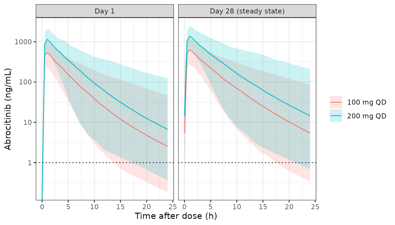
Median and 90% interval of simulated concentrations on day 1 and day 28; the dotted line is the 1 ng/mL lower limit of quantification. The paper’s own prediction-corrected VPC (Figure 2) uses the analysis dataset, which is not public, so it is not reproduced here.
PKNCA validation
PKNCA is run on the steady-state (day 28) interval of the cohort above, by dose group, and on a cohort of 200 White, male, adult, 80 kg atopic-dermatitis patients at 200 mg once daily with random effects. The latter matches the typical patient for which the paper reports a steady-state Cmax of 1123 ng/mL and AUC of 5662 ng h/mL (Results 3.4).
ref_cov <- reference_covariates(WT = 80, DIS_ATOPIC_DERMATITIS = 1)
obs_ref <- seq(27 * 24, 28 * 24, by = 0.25)
events_ref <- dplyr::bind_rows(lapply(seq_len(n_per_arm), function(i) {
  regimen_events(2L * n_per_arm + i, ref_cov, n_dose = 28, obs_times = obs_ref)
})) |>
  dplyr::mutate(treatment = "200 mg QD, White male 80 kg AD")
sim_ref <- rxode2::rxSolve(mod, events_ref, keep = "treatment", returnType = "data.frame")

conc_all <- dplyr::bind_rows(sim, sim_ref) |>
  dplyr::filter(!is.na(Cc)) |>
  dplyr::select(id, time, Cc, treatment)
dose_all <- dplyr::bind_rows(events, events_ref) |>
  dplyr::filter(evid == 1, cmt == "depot") |>
  dplyr::select(id, time, amt, treatment)

nca_res <- PKNCA::pk.nca(PKNCA::PKNCAdata(
  PKNCA::PKNCAconc(conc_all, Cc ~ time | treatment + id),
  PKNCA::PKNCAdose(dose_all, amt ~ time | treatment + id),
  intervals = data.frame(
    start = 27 * 24, end = 28 * 24,
    cmax = TRUE, tmax = TRUE, auclast = TRUE, cmin = TRUE
  )
))

as.data.frame(nca_res) |>
  dplyr::filter(PPTESTCD %in% c("cmax", "tmax", "auclast", "cmin")) |>
  dplyr::group_by(treatment, PPTESTCD) |>
  dplyr::summarise(median = signif(median(PPORRES), 3), .groups = "drop") |>
  tidyr::pivot_wider(names_from = PPTESTCD, values_from = median) |>
  dplyr::rename(
    "Group" = treatment,
    "Cmax (ng/mL)" = cmax,
    "Tmax (h)" = tmax,
    "AUC0-24 (ng*h/mL)" = auclast,
    "Cmin (ng/mL)" = cmin
  ) |>
knitr::kable(caption = "Median steady-state (day 28) NCA by group.")| Group | AUC0-24 (ng*h/mL) | Cmax (ng/mL) | Cmin (ng/mL) | Tmax (h) |
|---|---|---|---|---|
| 100 mg QD | 3070 | 635 | 5.42 | 1 |
| 200 mg QD | 6670 | 1360 | 14.50 | 1 |
| 200 mg QD, White male 80 kg AD | 6000 | 1130 | 15.20 | 1 |
Comparison against published NCA
published_nca <- tibble::tribble(
  ~treatment, ~cmax, ~auclast,
  "200 mg QD, White male 80 kg AD", 1123, 5662
)

cmp <- nlmixr2lib::ncaComparisonTable(
  simulated = nca_res,
  reference = published_nca,
  by = "treatment",
  units = c(cmax = "ng/mL", auclast = "ng*h/mL"),
  tolerance_pct = 20
)
knitr::kable(
  cmp,
  caption = "Simulated (median) vs. published steady-state exposure for the typical White adult atopic-dermatitis patient (80 kg, 200 mg QD). * differs from the reference by >20%."
)| NCA parameter | treatment | Reference | Simulated | % diff |
|---|---|---|---|---|
| Cmax (ng/mL) | 200 mg QD, White male 80 kg AD | 1120 | 1130 | +1.0% |
| AUClast (ng*h/mL) | 200 mg QD, White male 80 kg AD | 5660 | 6000 | +5.9% |
ref_nca <- as.data.frame(nca_res) |>
  dplyr::filter(treatment == "200 mg QD, White male 80 kg AD")
med_auc <- median(ref_nca$PPORRES[ref_nca$PPTESTCD == "auclast"])
med_cmax <- median(ref_nca$PPORRES[ref_nca$PPTESTCD == "cmax"])
typ_ad <- typ[typ$scenario == "AD, White, 80 kg", ]
stopifnot(
  # Deterministic: the typical-value AUC is F * dose / CL, which the paper
  # reports to four figures.
  abs(typ_ad$auclast / 5662 - 1) < 0.01,
  abs(typ_ad$cmax / 1123 - 1) < 0.05,
  # Cohort medians of 200 subjects: with 57.7% CV on CL the median AUC has a
  # sampling error of about 5%, so the bound allows three of those.
  abs(med_auc / 5662 - 1) < 0.20,
  abs(med_cmax / 1123 - 1) < 0.20
)
The typical-value AUC (5663 ng h/mL) matches the paper’s 5662 ng h/mL to within rounding. The typical-value Cmax (1099 ng/mL) is about 2% below the published 1123 ng/mL, consistent with the published value coming from a simulation that included random effects on Vc.
Assumptions and deviations
-
Two dose records per administration. The model
needs a
depotrecord (rate = 0) and acentralrecord (rate = -1) with the sameamt, as in the source dataset (Online Resource 2CMT/RATEdefinitions). rxode2 keeps the modelled rate and letsf(central)shorten the infusion, as NONMEM does. When the whole dose fits under the first-order cap (any tablet dose up to 121 mg) the central record carries no drug, and the model then drops its absorption lag; this changes nothing physically and avoids an rxode2 solver failure on lagged zero-amount infusions. -
Time on treatment. The source drives the
time-dependent clearance with
TAFO, the time after the first dose of a treatment period, which resets after a washout. The model uses the solver timet, so each treatment period must start att = 0; simulate crossover periods as separate subjects. NONMEM evaluates$PKonly at data records, so its clearance is piecewise constant between records, while rxode2 updates it continuously. -
Repeated-dosing flag.
MULTI_DOSEis 0 for single doses and for the first dose of a regimen and 1 from the second dose on (“single or first dose vs. multiple dosing”, Results 3.2). The source dataset carries the flag as a column; how its first-dose records were coded is not stated. -
Covariate coding. The five-level patient type
(
PTST) is split intoDIS_PSORIASIS,DIS_ATOPIC_DERMATITIS,HEPIMP_MILDandHEPIMP_MOD(all 0 = healthy volunteer), which are mutually exclusive. The four-level formulation (FORMS) is split into three indicators; with all three at 0 the dose is the phase II 100 mg tablet, which is the reference of every formulation effect in the control stream. The paper’s simulation reference is the phase III tablet (FORM_ABROCITINIB_TAB_PH3 = 1). The fluconazole and fluvoxamine shift on F applies once if either drug is present. Food-not-controlled records (FOOD = 2) are grouped with fasted, as in the control stream. -
800 mg dose. The -0.778 shift on logit F applies
when
DOSE_ABROCITINIB_MGis exactly 800 mg, as in the control stream (DOSE.EQ.800); it is not extrapolated to larger doses. - Female sex. The model keeps the published +0.353 logit-F shift, which does not reproduce the near-unity Female row of Figure 3 (see above).
- Censoring. The paper fitted below-quantification concentrations with the M3 method (LLOQ 1 ng/mL); that affects estimation only, and simulations here return uncensored concentrations.
-
Units. Table 2 prints the maximum time-dependent
change in CL as “-0.186 %”; the control stream uses it as a fraction
(
1 + TAFOCLDELTA * (1 - exp(...))), so CL falls by 18.6% at steady state. - Virtual cohort. The atopic-dermatitis covariate distribution is an approximation of Table 1 (independent sampling, log-normal weight); it is used only for the illustrative percentile plot and the per-dose NCA.